
Non-contact river discharge vs ADCP: DoorDrishti in a Himalayan field test
DoorDrishti measured river discharge from a bridge without touching the water. We checked it against boat-mounted ADCP gaugings on two days, a month apart, at very different flows.

How accurate is non-contact river discharge measurement? It is the first question every hydrologist asks, and the right one. A sensor that never touches the water is safe to install and keeps working through a flood, but it has to earn trust against the methods engineers already rely on.
So we tested ours. On a mountain river in Mandi district, Himachal Pradesh, a DoorDrishti test installation on a road bridge measured discharge through the 2026 monsoon. On two days, a team gauged the same river with an acoustic Doppler current profiler (ADCP) from a moving boat. This case study puts the two side by side.
The short answer: on 21 August DoorDrishti's discharge was 5 % above the ADCP's, and on 18 September, at half the flow, 7 % above. Both are close to the spread of the ADCP gauging itself. Below we explain what we measured, how we compared it, and what the difference means.
What is non-contact discharge measurement?
Discharge is the volume of water passing a section each second, in cubic metres per second (m³/s). The standard way to get it is the velocity–area method: divide the river into vertical slices, measure the depth and the average velocity in each, multiply and add up [1].
A non-contact system does the same sum without putting anything in the water:
- Water level comes from a radar looking straight down at the surface. With a surveyed cross-section, level gives the wetted area.
- Surface velocity comes from a radar that measures the Doppler shift of ripples on the surface, or from a camera that tracks how surface patterns move between video frames. The camera methods are known as image velocimetry; the best known is large-scale particle image velocimetry (LSPIV) [2][3].
- Average velocity in each slice is lower than the surface velocity, because water slows towards the bed. A site-calibrated coefficient links the two.
We explain the radar side in more detail in Can radar measure river discharge? and the camera side in camera-based river monitoring.
The site
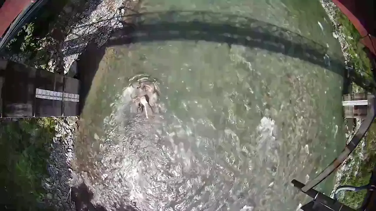
The river is a steep, boulder-bed Himalayan stream, typical of the hill rivers that carry flash floods in Himachal Pradesh. At the bridge it is about 40 m wide and mostly less than a metre deep during the monsoon, with fast, broken water over boulders.
- DoorDrishti's radar and camera sit on a road bridge, about 13 metres above the water.
- The radar records water level and surface velocity every 15 minutes; the camera records short videos through the day.
- Water level is referred to a surveyed datum, and the cross-section under the bridge was surveyed.
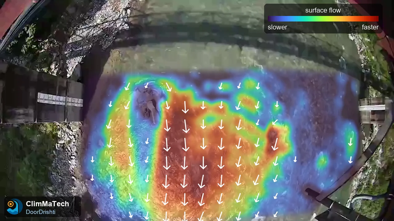
DoorDrishti combines the two: the camera sees the whole width of the river, and the radar gives a continuous, light-independent reference. How they are combined is ClimMaTech's own method; we do not describe it here.
How did we compare with the ADCP?
An ADCP measures water velocity through the whole depth from a boat crossing the river, and adds up discharge directly. It is the accepted reference for gauging rivers of this size [4]. Each crossing is called a transect, and a gauging is normally the average of several transects.
- The ADCP gaugings were made upstream of the bridge, where the river is deeper and calmer and the boat could cross safely. No stream joins between the two sections, so the discharge is the same.
- We counted only transects that crossed the full width of the river. For the narrow strip beside a vertical rock bank, which the boat could not reach, we added the standard edge estimate [4].
- 21 August 2026: three transects between 12:42 and 13:03.
- 18 September 2026: four full-width crossings (two boat runs, each across and back) between 15:46 and 15:54.
- For each day we took DoorDrishti's discharge for the same time window.
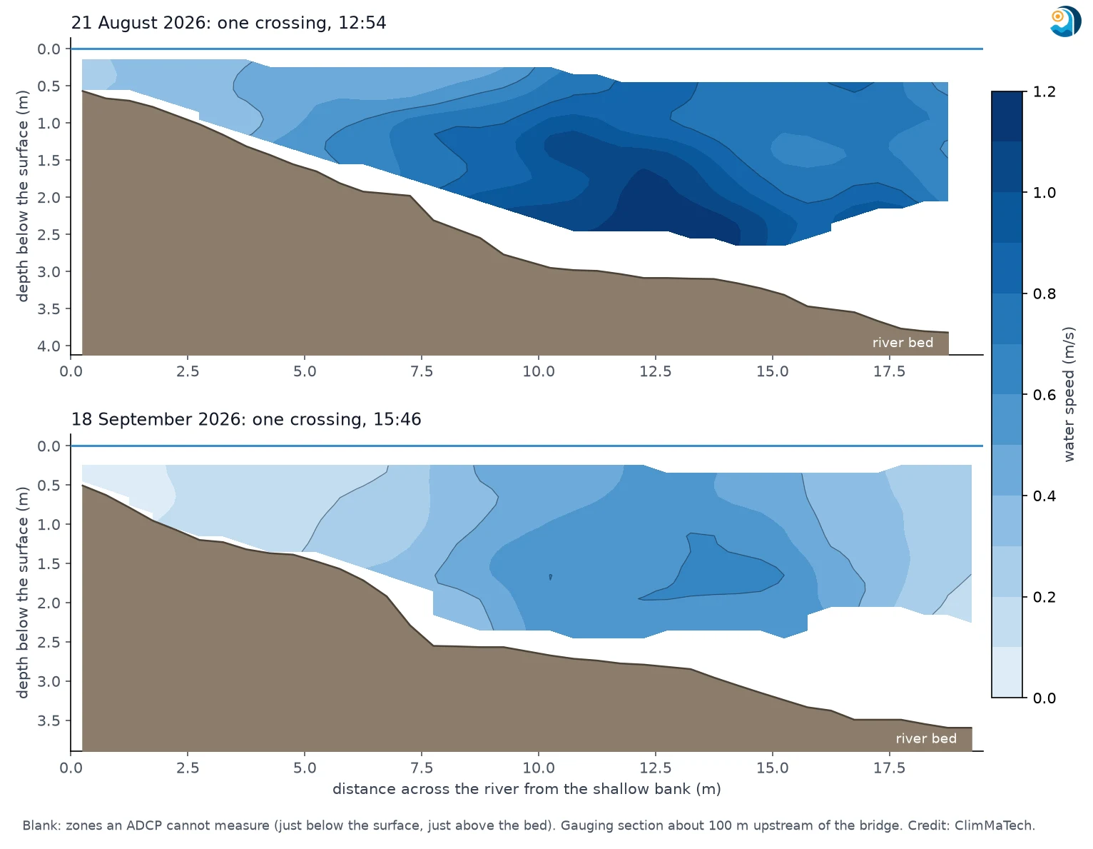
One point matters for a fair comparison: an ADCP gauging has its own spread. Transects on the same day, minutes apart, rarely agree exactly. On 18 September our four crossings ranged from 16.0 to 17.6 m³/s, including the edge allowance, a spread of about ±5 %. On 21 August the three transects ranged from 32.3 to 33.1 m³/s. Under good conditions, a single discharge measurement by conventional methods is typically uncertain by 3–6 % [5]. That is the yardstick any other method should be judged against.
Results
DoorDrishti is set up at a site with one survey day, on which the surface velocity across the river is measured by hand. To show how much the choice of that day matters, we repeated the set-up with each survey day we made in August and September and report the median and the range. One survey failed a quality check and was not used.
| Date | Time | ADCP transects | ADCP discharge (m³/s) | ADCP spread | DoorDrishti discharge (m³/s) | DoorDrishti range | Difference |
|---|---|---|---|---|---|---|---|
| 21 Aug 2026 | 12:42–13:03 | 3 | 32.7 | ±1.2 % | 34.2 | 32.5–37.8 | +5 % |
| 18 Sep 2026 | 15:46–15:54 | 4 | 16.8 | ±5 % | 17.9 | 16.9–19.9 | +7 % |
21 August: higher flow
The ADCP gave 32.7 m³/s, the mean of three transects (32.3 to 33.1 m³/s), and DoorDrishti 34.2 m³/s, 5 % higher. That is within the 3–6 % uncertainty normally expected of a single conventional discharge measurement [5]. Depending on the survey day used for set-up, DoorDrishti's value ranged from 1 % below to 16 % above the ADCP.
18 September: half the flow
The ADCP gave 16.8 m³/s, the mean of four crossings, and DoorDrishti 17.9 m³/s, 7 % higher, with a range of 0 % to 18 % above the ADCP across the survey days. The station's last reading that day was at 13:00, about three hours before the gauging. The river had been steady all morning, changing by less than 2 % between 10:00 and 13:00, so we compared with that value. The difference is a little larger than the ADCP's own ±5 % spread.
On both days DoorDrishti read slightly high, and the same survey days gave the highest values on both. That points to the set-up survey, not the sensor, as the main source of the spread, and to a simple remedy: a second survey day at a different flow.
What did the station see that the gaugings did not?
A gauging is a snapshot. DoorDrishti measures all day.
On 21 August the river was falling. DoorDrishti's discharge dropped from about 39 m³/s in the early hours to about 30 m³/s by midnight, a fall of about a fifth in one day. The midday gauging caught one point on that fall. DoorDrishti recorded the whole of it, including the night, when no one can gauge a mountain river safely.
How accurate is non-contact discharge measurement in general?
Published comparisons of surface velocity radar and image velocimetry with ADCPs and current meters report differences from a few per cent at well-suited sites to 15–20 % or more under difficult conditions [3][6][7]. Three things decide where a given site falls:
- The cross-section. Area errors pass straight into discharge. A good, recent survey matters as much as the velocity sensor.
- The surface-to-average velocity coefficient. It depends on the depth and the roughness of the bed and is best set from gaugings at the site. On its own it can shift discharge by up to about 10 % [3].
- Conditions at the surface. Low sun, shadows, glare and rain affect a camera; wind on the surface affects a radar. Using both, and knowing when each is reliable, is what keeps the record usable.
Limits of this test
- Two gaugings at one site. That is a start, not a full validation.
- The ADCP worked upstream of the bridge, not at the same section.
- On 18 September the comparison relies on the river staying steady between the station's last reading at 13:00 and the gauging about three hours later.
- The comparison covers moderate monsoon flows of about 17 to 33 m³/s. Higher flows were measured by DoorDrishti but not gauged.
- DoorDrishti's values depend on which survey day is used for set-up; we report the median and the range over the survey days available.
Key points
- DoorDrishti, mounted on a bridge, measured discharge on a Himalayan river without touching the water, through the 2026 monsoon.
- Against boat-mounted ADCP gaugings, DoorDrishti's discharge was 5 % higher at 33 m³/s and 7 % higher at 17 m³/s.
- Both are close to the uncertainty of a single conventional gauging. Most of the remaining spread comes from the one-day site set-up, which a second survey at a different flow would narrow.
- DoorDrishti adds what a gauging cannot: a continuous record, including nights and falling or rising water.
- Accuracy depends as much on the cross-section survey and site calibration as on the sensor.
About this work
This test was run by ClimMaTech at its own installation. DoorDrishti combines radar water level and surface velocity sensing (the same radar as in PRAVAAH) with an AI camera in one unit; with a surveyed cross-section and site calibration, it reports discharge without touching the water. For a site assessment, see our river monitoring solution.
Method
Station: DoorDrishti test installation (radar water level and surface velocity, and camera) on a road bridge about 13 m above the water. The radar records every 15 minutes; camera videos are recorded through the day. Water level is referred to a surveyed datum. Discharge is computed by the velocity–area method over the surveyed cross-section with a site-calibrated surface-to-average velocity coefficient.
Reference: moving-boat ADCP gaugings with a multi-frequency ADCP with bottom tracking and RTK GPS. Transects used: three on 21 August (one recorded with a wrong sensor-depth setting, recomputed from the raw data with the correct setting) and four full-width crossings on 18 September. Edge discharge beside the banks was estimated with the standard edge method [4]. The reference discharge is the mean of the transects, and the spread is the range across them.
Comparison: DoorDrishti's discharge for the gauging time (21 August: the mean of the 15-minute values inside the gauging window; 18 September: the last reading of the day, 13:00, with the river steady through the morning); difference = (DoorDrishti − ADCP) / ADCP. DoorDrishti was set up with one survey day at a time (six survey days for 21 August, seven for 18 September, excluding the gauging day itself and one survey that failed a quality check); we report the median and the range.
References
- International Organization for Standardization, ISO 748:2021 Hydrometry — Measurement of liquid flow in open channels — Velocity-area methods using point velocity measurements, ISO, 2021. https://www.iso.org/standard/76960.html
- Fujita, I., Muste, M. and Kruger, A., Large-scale particle image velocimetry for flow analysis in hydraulic engineering applications, Journal of Hydraulic Research 36(3), 397–414, 1998. https://doi.org/10.1080/00221689809498626
- Le Coz, J., Hauet, A., Pierrefeu, G., Dramais, G. and Camenen, B., Performance of image-based velocimetry (LSPIV) applied to flash-flood discharge measurements in Mediterranean rivers, Journal of Hydrology 394, 42–52, 2010. https://doi.org/10.1016/j.jhydrol.2010.05.049
- Mueller, D.S., Wagner, C.R., Rehmel, M.S., Oberg, K.A. and Rainville, F., Measuring discharge with acoustic Doppler current profilers from a moving boat (ver. 2.0), U.S. Geological Survey Techniques and Methods 3-A22, 2013. https://doi.org/10.3133/tm3A22
- Fulton, J.W., Mason, C.A., Eggleston, J.R., et al., Near-field remote sensing of surface velocity and river discharge using radars and the probability concept at 10 U.S. Geological Survey streamgages, Remote Sensing 12(8), 1296, 2020. https://doi.org/10.3390/rs12081296
- Costa, J.E., Cheng, R.T., Haeni, F.P., et al., Use of radars to monitor stream discharge by noncontact methods, Water Resources Research 42, W07422, 2006. https://doi.org/10.1029/2005WR004430
- Welber, M., Le Coz, J., Laronne, J.B., et al., Field assessment of noncontact stream gauging using portable surface velocity radars (SVR), Water Resources Research 52, 1108–1126, 2016. https://doi.org/10.1002/2015WR017906