
The velocity-area method: how rivers are gauged by hand
How a hydrographer turns depths and point velocities across a river into one discharge figure, with a fully worked example and what changes in a monsoon flood.

Almost every discharge figure in a river record traces back to a few days when someone went to the river and measured it. A level sensor records stage, and a rating curve converts stage to discharge. The rating curve is built from gaugings, direct measurements of discharge made at different stages, and most gaugings are made with the velocity-area method. If you use discharge data, it helps to know how the number was produced and how far to trust it. This article walks through a gauging from start to finish, with a fully worked example, the main sources of error, and the conditions Indian field teams face in the monsoon.
The idea in one line
Discharge Q (m³/s) is the volume of water passing a cross-section each second: area times mean velocity. Velocity varies across the river and from surface to bed, so the method divides the cross-section into narrow panels (also called segments or partial sections), measures a depth and a mean velocity for each, and adds up the panel discharges:
Q = Σ q(i) = Σ v(i) × a(i)where a(i) is the area of panel i and v(i) the mean velocity normal to the section in it. The international standard is ISO 748, now in its 2021 edition. It covers rotating-element current meters, acoustic Doppler velocimeters, stationary acoustic Doppler current profilers and surface velocity methods including floats [1]. Field practice is described in the WMO Manual on Stream Gauging [2], the USGS manual by Turnipseed and Sauer [3] and the Central Water Commission (CWC) field manual [4].
Step 1: choose the measuring section
At a cableway the section is fixed. When wading or using a boat, the hydrographer looks for the qualities that ISO 748 lists, as summarised in the WMO Manual [2]:
- a straight reach of uniform section and slope;
- a stable bed free of large rocks, weeds and obstructions that create eddies or slack water;
- no reverse flow, vortices, dead water, or converging or diverging flow;
- enough depth at all stages to submerge the meter;
- safe access at all times, close to the gauge and its control with no tributary in between.
Few sections meet all of these, so the aim is the best reach available [2]. CWC allows a wading section to be several hundred metres from the staff gauges if no water enters or leaves in between [4].
Step 2: lay out the verticals
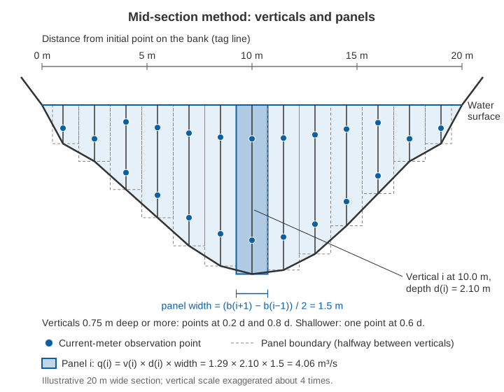
A tag line or tape is stretched across the river at right angles to the flow, and positions are measured from an initial point on the bank. Each vertical is a line from surface to bed where depth and velocity are measured; the water's edge is the first.
How many? WMO and USGS generally use 25 to 30 partial sections on streams wider than about 10 m, spaced so that no partial section carries more than 10 % of the total discharge, ideally no more than 5 % [2][3]. CWC asks for at least 20 verticals, normally 20 to 30, on rivers wider than 10 m, with the same 10 % limit. It gives a table for narrower channels, from 3 to 4 verticals under 0.5 m width up to 20 at 10 m, and adds that depths at adjacent verticals should not differ by more than 50 % of the smaller [4].
Equal spacing is not recommended unless flow is very evenly spread: verticals should be closer where depth and velocity are greater. A useful trick is to read an approximate discharge from the rating curve before starting, then aim for about 5 % of it per panel [2].
Step 3: measure the depth
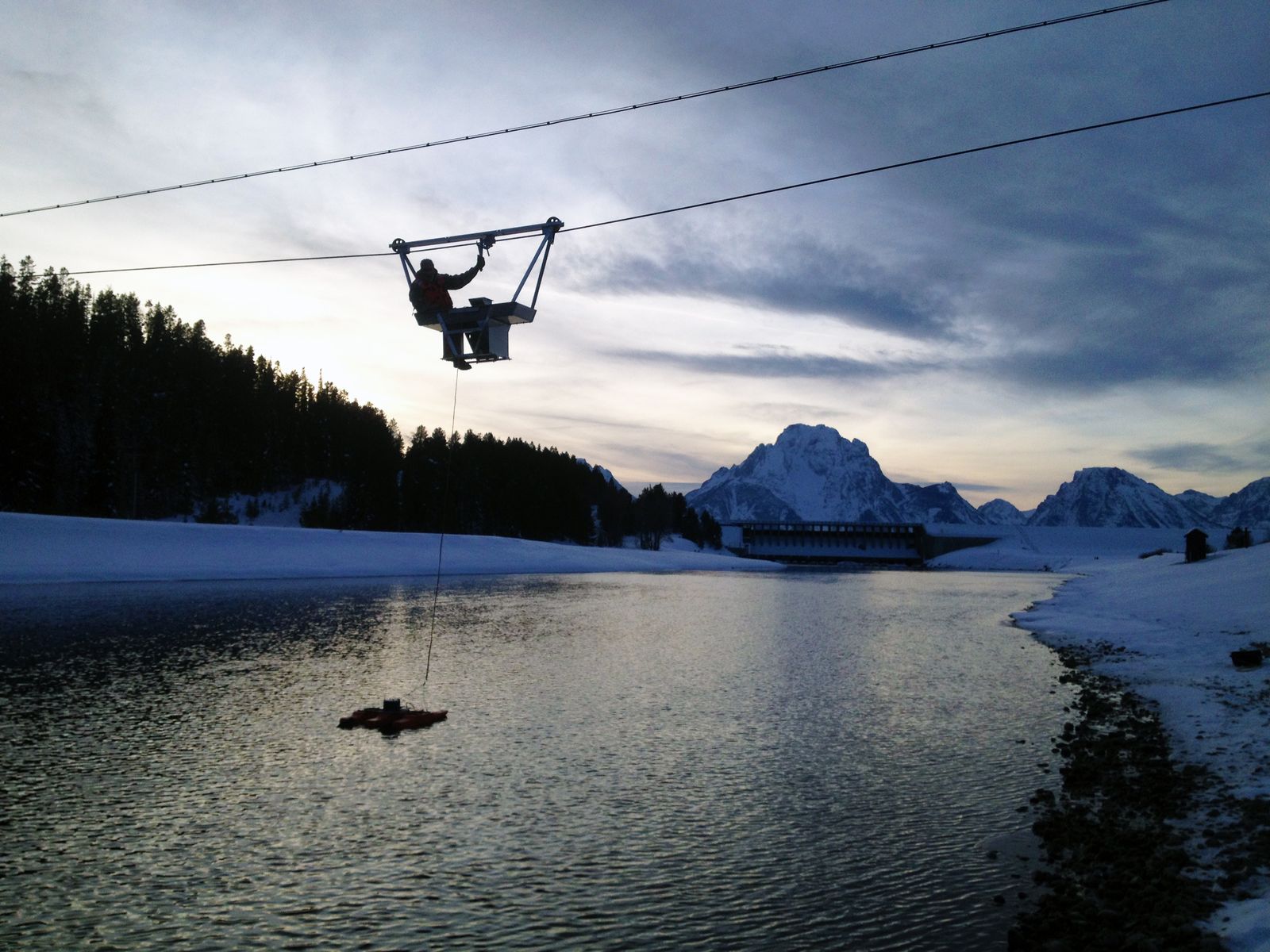
When wading, depth is read from a graduated rod, usually to the nearest 5 mm. From a bridge, cableway or boat, a sounding weight hangs below the meter on a cable, keeping it steady and protecting it at the bed. CWC's rule of thumb is a weight in kg of more than 5 times velocity (m/s) times depth (m) [4]: at 2 m/s and 3 m depth, more than 30 kg. In deep, fast water the weight is swept downstream and the cable leans, so the cable paid out is longer than the true depth. The hydrographer reads the cable angle with a protractor and applies air-line and wet-line corrections from tables [2][4].
Step 4: measure velocity at the right points
A current meter measures velocity at a point, but we need the mean velocity in the vertical. Velocity is lowest near the bed and highest near the surface, and in a normal profile the mean lies at about 0.6 of the depth below the surface. The standard methods use this shape [2][4]:
| Method | Meter position (fraction of depth below surface) | Mean velocity | Typical use |
|---|---|---|---|
| Two-point | 0.2 and 0.8 | Average of the two | Depths of 0.75 m or more (WMO); CWC uses it above 1.0 m |
| Six-tenths | 0.6 | The reading itself | Depths of about 0.1 to 0.75 m; rapidly changing stage |
| Three-point | 0.2, 0.6 and 0.8 | Mean of the 0.2/0.8 average and the 0.6 reading | Abnormal profiles |
| Two-tenths | 0.2 | Reading × about 0.87 | Floods, when the meter cannot reach deeper |
| Surface | Surface (float, optical meter, radar) | Reading × about 0.84 to 0.90 | Deep, swift or dangerous flow |
According to the WMO Manual, the two-point method averages within 1 % of the true mean when the profile is roughly parabolic. A quick check: the 0.2-depth velocity should exceed the 0.8-depth velocity but be less than twice it; if not, add a reading at 0.6 depth [2]. The surface coefficient is higher over smooth beds and lower over irregular ones [2]. CWC uses 0.85 unless gaugings at the site show otherwise [4], and site-measured velocity profiles are the best basis. The same question arises with radar, discussed in surface velocity radar for rivers. A standard 100 mm meter should not normally be used in water shallower than about 0.4 m (four rotor diameters) [4].
Step 5: the current meter, its rating and exposure time
A rotating-element current meter, either cup-type or propeller, spins at a rate that depends on water speed. A rating equation, usually of the form v = a·n + b with n in revolutions per second, converts the count into velocity. The constants come from a towing tank: a carriage tows the meter through still water at accurately measured speeds, typically from about 0.1 to 4 m/s in tanks 50 to 200 m long [2]. Some meters are rated individually, others share a standard rating for identically built meters [3]. Record the rating number and date, and do a spin test before and after each gauging, by blowing on the rotor rather than turning it by hand, which can damage the bearings [4].
The counting interval is the exposure time. Velocity at a point fluctuates (pulsation), so a longer count gives a better average. WMO and USGS count for 40 to 70 seconds [2][3]. CWC recommends 60 seconds in most Indian conditions, 100 seconds if there are fewer than 20 revolutions in 50 seconds, and as little as 30 seconds when stage is changing fast [4].
Illustrative example. Take a rating of v = 0.25·n + 0.015. At 0.2 depth the meter makes 356 revolutions in 60 s: n = 5.933, so v = 0.25 × 5.933 + 0.015 = 1.50 m/s. At 0.8 depth, 256 revolutions give n = 4.267 and v = 1.08 m/s. The mean in the vertical is (1.50 + 1.08) / 2 = 1.29 m/s, and the ratio 1.50 / 1.08 = 1.39 passes the WMO check.
Step 6: compute discharge by the mid-section method
In the mid-section method, the standard in CWC practice, each vertical represents a rectangular panel reaching halfway to the neighbouring verticals and down to the measured depth [2][4]:
q(i) = v(i) × d(i) × [ b(i+1) − b(i−1) ] / 2where b is distance from the initial point and d(i) the depth. At a sloping bank the edge depth is zero and the end panel adds nothing. At a wall, abutment or pier, the edge velocity is usually estimated as a percentage of that at the nearest vertical [2][4].
A fully worked example
The numbers are illustrative: a 20 m wide section gauged with 13 verticals, deliberately few so the arithmetic fits on the page. Verticals 0.75 m deep or more use the two-point method, shallower ones 0.6 depth.
| Distance b (m) | Depth d (m) | v at 0.2d / 0.8d or 0.6d (m/s) | Mean v (m/s) | Panel width (m) | Area (m²) | q (m³/s) | Share of Q |
|---|---|---|---|---|---|---|---|
| 0.0 (edge) | 0.00 | – | 0 | 0.50 | 0.000 | 0.000 | 0 % |
| 1.0 | 0.48 | 0.40 (0.6d) | 0.40 | 1.25 | 0.600 | 0.240 | 0.9 % |
| 2.5 | 0.70 | 0.55 (0.6d) | 0.55 | 1.50 | 1.050 | 0.578 | 2.2 % |
| 4.0 | 1.05 | 0.86 / 0.60 | 0.73 | 1.50 | 1.575 | 1.150 | 4.4 % |
| 5.5 | 1.40 | 1.12 / 0.80 | 0.96 | 1.50 | 2.100 | 2.016 | 7.7 % |
| 7.0 | 1.75 | 1.32 / 0.94 | 1.13 | 1.50 | 2.625 | 2.966 | 11.3 % |
| 8.5 | 2.00 | 1.45 / 1.05 | 1.25 | 1.50 | 3.000 | 3.750 | 14.3 % |
| 10.0 | 2.10 | 1.50 / 1.08 | 1.29 | 1.50 | 3.150 | 4.064 | 15.5 % |
| 11.5 | 2.05 | 1.46 / 1.06 | 1.26 | 1.50 | 3.075 | 3.875 | 14.8 % |
| 13.0 | 1.85 | 1.36 / 0.98 | 1.17 | 1.50 | 2.775 | 3.247 | 12.4 % |
| 14.5 | 1.50 | 1.18 / 0.84 | 1.01 | 1.50 | 2.250 | 2.273 | 8.7 % |
| 16.0 | 1.10 | 0.92 / 0.66 | 0.79 | 1.50 | 1.650 | 1.304 | 5.0 % |
| 17.5 | 0.70 | 0.54 (0.6d) | 0.54 | 1.50 | 1.050 | 0.567 | 2.2 % |
| 19.0 | 0.48 | 0.38 (0.6d) | 0.38 | 1.25 | 0.600 | 0.228 | 0.9 % |
| 20.0 (edge) | 0.00 | – | 0 | 0.50 | 0.000 | 0.000 | 0 % |
| Total | 20.0 | 25.50 | 26.26 | 100 % |
At 10.0 m: panel width = (11.5 − 8.5) / 2 = 1.5 m; area = 1.5 × 2.10 = 3.15 m²; mean velocity = 1.29 m/s; panel discharge = 3.15 × 1.29 = 4.06 m³/s. The panel at 1.0 m is (2.5 − 0) / 2 = 1.25 m wide. Summing all panels gives Q = 26.26 m³/s through 25.50 m², a mean velocity of 1.03 m/s.
The table also shows the gauging's weakness: five panels each carry more than 10 % of the flow, the largest 15.5 %. Equal 1.5 m spacing leaves too few verticals where the river is deep and fast. Adding a vertical midway between each pair from 5.5 m to 14.5 m would roughly halve those shares and give 22 verticals, within CWC's range of 20 to 30 [4].
Mean-section method, for comparison
The mean-section method sets panels between adjacent verticals, multiplying the average of their velocities by the average of their depths and the distance between them [2]:
q(i, i+1) = [ (v(i) + v(i+1)) / 2 ] × [ (d(i) + d(i+1)) / 2 ] × [ b(i+1) − b(i) ]Between 8.5 m and 10.0 m: 1.27 × 2.05 × 1.5 = 3.905 m³/s. Over the whole table the mean-section method gives 25.95 m³/s, 1.2 % less than mid-section, from the same 25.50 m² of area. The WMO Manual cites a study by Young (1950) that found the mid-section method simpler and slightly more accurate, as ISO 748 also concludes [2].
Try it yourself
Change the depth or velocity of any of the five verticals below. With only five, at least one panel always carries 20 % of the flow or more, and the two computation methods drift apart.
The calculator's channel and values are illustrative.
How accurate is a gauging?
ISO 748 splits the uncertainty of a gauging into components, each a percentage standard uncertainty (about 68 % confidence). The WMO Manual gives guide values, following the 2007 editions of ISO 748 and ISO 1088 [2]:
- u_m, number of verticals: 7.5 % with 5 verticals, 2.5 % with 20, 1.0 % with 35 or more.
- u_p, points in the vertical: about 3.5 % for two-point, 7.5 % for 0.6 depth, 15 % for a surface reading.
- u_e, exposure time: at 0.1 m/s and 0.2 depth, 11 % for a 1-minute count and 7 % for 3 minutes; a few percent above 0.3 m/s.
- u_c, meter rating: for an individually rated meter, about 0.5 % above 0.5 m/s but 10 % at 0.03 m/s.
- u_b, u_d, u_s: width, depth and systematic terms.
They combine, for m verticals with n points each, as:
u(Q) = √[ u_s² + u_m² + (1/m) × ( u_b² + u_d² + u_p² + (1/n) × (u_c² + u_e²) ) ]The WMO example (20 verticals, two points, 0.3 m/s, 3-minute counts, individual rating) uses u_m = 2.5, u_s = 1.0, u_b = u_d = 0.5, u_p = 3.5, u_c = 0.9 and u_e = 4.2, giving u(Q) = √(2.5² + 1² + (0.5² + 0.5² + 3.5² + (0.9² + 4.2²) / 2) / 20) ≈ 2.9 % [2]. The same numbers with 10 verticals (u_m = 4.5) give about 4.8 %. The number of verticals is the largest term in both.
CWC's conclusion is practical: it is better to use more verticals than to measure more points in each [4]. Research agrees and goes further. Le Coz and co-authors proposed a more general uncertainty method that accounts for edge and top/bottom extrapolation and for where the verticals are placed; it matched ISO 748 on standard natural sections but differed for regular man-made canals [5]. Despax and co-authors noted that ISO 748's u_m depends only on how many verticals are used, not where. Across 3,185 gaugings, an index of how well the verticals sample the section explained uncertainty better than their number alone [6]. Pelletier's review of more than 140 publications catalogued the error sources of a single current-meter measurement [7].
USGS also rates each measurement by conditions on the day: excellent (2 %), good (5 %), fair (8 %) or poor (more than 8 %) [3]. These uncertainties carry straight into the rating curve, as discussed in rating curves: from stage to discharge.
Gauging Indian rivers in the monsoon
The method is simple on a calm day in a wadeable stream. In a monsoon flood, the CWC field manual addresses the main problems directly [4]:
- Cableways and bridges. The upstream side of a bridge usually has better flow, less scour and a clear view of approaching drift. The downstream side makes cable angles easier to read and suffers less from debris piled on piers. Where each span acts as its own channel, take five verticals per span if possible and never fewer than three. Set up warning signs and cones for road traffic.
- Debris. Raise and clean the meter whenever the count drops suddenly. In extreme conditions one team member stands by with wire cutters, ready to cut the cable if a tree trunk snags the assembly and endangers the cableway and crew.
- Oblique flow. Cable-suspended meters align with the current, so where the section is not square to the flow, multiply velocity by the cosine of the flow angle.
- Rapidly changing stage. If stage changes by more than 0.05 m during the gauging, use a discharge-weighted mean gauge height. In a rising flood, a quick gauging under 30 minutes is allowed: 30-second counts, 0.2-depth readings multiplied by 0.87 (or a site value), and depths from a pre-surveyed section.
- Boats. Everyone wears a life jacket, one person only controls the boat, and no gauging is done within 500 m upstream of a weir, sluice, waterfall or rapids without special safety measures.
When a meter cannot go in the water, CWC uses floats: wooden rods 0.4 m long and 4 cm across, weighted to float upright with a third above water [4]. The timed reach is 3 to 5 times the river width, or at least 20 seconds of travel, between two surveyed sections that are resurveyed at least once a year before the monsoon. Floats are released at an odd number of positions, usually no more than seven. Mean velocity is taken as 0.85 times surface velocity unless gaugings at the site support another value. USGS puts float measurements under favourable conditions within about ±10 % and warns that wind can degrade them [3]. Drift often eases soon after the crest, which may allow current-meter readings that help set the coefficient [2].
These hazards are why most gaugings are made at moderate flows and why the top of a rating curve is so often extrapolated. Non-contact surface velocity methods are one way to fill that gap; see can radar measure river discharge?
Key points
- Discharge is the sum of depth × width × mean velocity over many narrow panels.
- Use 20 to 30 verticals on rivers wider than about 10 m, with no panel carrying more than 10 % of the flow.
- Measure at 0.2 and 0.8 depth in deeper water and 0.6 depth in shallow water; surface readings need a coefficient, best set at the site.
- Count for about 40 to 70 seconds (60 s in CWC practice) with a rated meter that has passed its spin test.
- The mid-section method is standard; the mean-section method gives slightly different totals.
- The number of verticals is usually the largest uncertainty term. A good current-meter gauging is uncertain by a few percent; float gaugings are within about 10 % at best.
Careful gaugings remain the reference against which every level-based or surface-velocity discharge record is checked, and they are part of how we approach river stations at ClimMaTech. See PRAVAAH, an AWLR (automatic water level recorder) and SVR (surface velocity radar) that gives discharge without contact once the cross-section is surveyed and the surface coefficient is calibrated at the site, and our river monitoring solutions.
References
- International Organization for Standardization, ISO 748:2021 Hydrometry — Measurement of liquid flow in open channels — Velocity area methods using point velocity measurements, ISO, 2021. iso.org.
- World Meteorological Organization, Manual on Stream Gauging, Volume I: Fieldwork, WMO-No. 1044, WMO, 2010, Chapters 5 and 10. wmo.int (PDF).
- D. P. Turnipseed and V. B. Sauer, Discharge Measurements at Gaging Stations, U.S. Geological Survey Techniques and Methods, book 3, chapter A8, 2010. doi.org/10.3133/tm3A8.
- Central Water Commission, Gauge & Discharge Measurement Field Manual, Volume 4 Hydrometry, Parts III (float measurements) and IV (current meter gauging), River Data Directorate, CWC, January 2005. cwc.gov.in (PDF).
- J. Le Coz, B. Camenen, X. Peyrard and G. Dramais, Uncertainty in open-channel discharges measured with the velocity–area method, Flow Measurement and Instrumentation 26, 18–29, 2012. doi.org/10.1016/j.flowmeasinst.2012.05.001.
- A. Despax, C. Perret, R. Garçon, A. Hauet, A. Belleville, J. Le Coz and A.-C. Favre, Considering sampling strategy and cross-section complexity for estimating the uncertainty of discharge measurements using the velocity-area method, Journal of Hydrology 533, 128–140, 2016. doi.org/10.1016/j.jhydrol.2015.11.048.
- J. M. Pelletier, Uncertainties in the single determination of river discharge: a literature review, Canadian Journal of Civil Engineering 15(5), 834–850, 1988. doi.org/10.1139/l88-109.