
Rain gauge density: how many gauges does a district need?
How to size a rain gauge network: WMO and BIS minimum densities, the optimum number formula N = (Cv/ε)², why hills need more gauges, and how to check the network you already have.

A district disaster management office is asked to strengthen its rainfall monitoring before the next monsoon. The first question is always the same: how many rain gauges does the district need, and where should they go? There are two standard answers. One is a table of rain gauge density, the area each gauge is expected to represent, published by the World Meteorological Organization (WMO) and, for India, by the Bureau of Indian Standards (BIS). The other is a statistical calculation, the optimum number of rain gauges, based on how much rainfall varies across the area. This article explains both, works through an illustrative district, and covers what the numbers leave out: hills, flood warning and checking an existing network.
A gauge measures rain at one point, but planners and forecasters usually want the areal mean rainfall, the average depth over a catchment or district. Each gauge is a sample of that average; more gauges reduce the uncertainty but cost more to install, read and maintain for decades. BIS names the orography of a place and the variability of rainfall there as the two most important factors in network design [2].
What is the rain gauge density as per WMO?
WMO gives recommended minimum densities of stations by physiographic unit in its Guide to Hydrological Practices, WMO-No. 168, Table I.2.6 [1]. Density is written as the area represented by one station, so a smaller number means a denser network:
| Physiographic unit | Non-recording gauges (km² per gauge) | Recording gauges (km² per gauge) |
|---|---|---|
| Coastal | 900 | 9,000 |
| Mountains | 250 | 2,500 |
| Interior plains | 575 | 5,750 |
| Hilly / undulating | 575 | 5,750 |
| Small islands | 25 | 250 |
| Urban areas | – | 10–20 |
| Polar / arid | 10,000 | 100,000 |
Source: WMO-No. 168, Volume I, Table I.2.6 [1]. A non-recording gauge is read by an observer, usually once a day; a recording gauge logs rainfall continuously, so it also gives intensity and timing.
- These are minimums. WMO says the densities must be adjusted to actual socio-economic and physio-climatic conditions, with mathematical analysis used where data allow [1]. They are a floor, not a design.
- Their basis. The values come from a 1991 review of member countries' responses to a WMO network assessment project [1]. Small islands are those under 500 km².
- Urban areas need a very dense network to resolve storms in space and time for storm-drain design and real-time control, at a time resolution of one to two minutes [1].
What rain gauge density does the IS code recommend?
The Indian standard is IS 4987:1994, *Recommendations for establishing network of raingauge stations* (first revision of the 1968 standard), which covers the distribution, density and representativeness of rain gauge networks; BIS lists it with no amendments [2]. It gives density guidance in two places.
Its guiding principles (clause 3) say [2]:
- Plains: one rain gauge for up to 500 km² is sufficient, but the network should be denser, particularly upstream, if the catchment lies in the path of the low pressure systems that bring its rain.
- Moderately elevated regions (average elevation about 1 km above sea level): one gauge per 250 to 400 km².
- Predominantly hilly areas with very heavy rainfall: one gauge in not more than 150 km², and denser if possible, except where the catchment lies in the rain shadow of high barriers.
For a minimum network, where even the optimum design is not feasible (clause 6.3) [2]:
| Terrain | IS 4987 minimum network (km² per gauge) |
|---|---|
| Plains | at least one gauge per 750 |
| Hilly regions | normally 100 to 250 |
| Arid areas | normally 1,500 to 10,000 |
IS 4987 also asks for an even spread, since a network dense in some parts and sparse in others biases the assessment. It suggests choosing stations whose Thiessen polygons (the area closer to each gauge than to any other) carry roughly equal weight, without dropping any station in a pocket of heavy rainfall [2].
What is the optimum number of rain gauges formula?
Density tables ignore how variable the rain is in your area; the optimum number formula uses it directly. IS 4987 (clause 5.2) gives it for a mean rainfall computed as the arithmetic average of the gauges [2]:
N = (Cv / ε)²

N  = optimum number of rain gauges
Cv = coefficient of variation of rainfall at the existing gauges, %
     = 100 × (standard deviation / mean)
ε  = acceptable error in the estimate of mean rainfall, %
IS 4987 writes the error as P and recommends estimating the mean within 10 %, noting that a smaller error means more gauges and higher operating cost [2].
The derivation shows the limits. If N gauges each give an independent sample of rainfall with standard deviation σ, the standard error of their average is σ/√N. Dividing by the mean gives a relative error ε = Cv/√N, and squaring gives N = (Cv/ε)². Three assumptions follow:
- ε is one standard error, not a worst case. If the errors are roughly normal, the true mean lies within ±ε about two times in three.
- The gauges are treated as independent. Nearby gauges are correlated, so a cluster of new gauges adds less information than assumed. Methods that include spatial correlation, measurement errors and site costs, and choose both number and location, date from the 1970s [4]; Mishra and Coulibaly review the field [9].
- Cv must come from the right rainfall. Annual totals vary much less across an area than single storms. Using two dense networks in Illinois, Huff found sampling requirements for monthly and seasonal rainfall substantially lower than for storms; warm-season storms needed two to three times the gauge density of cold-season storms, and unstable rainfall twice as many gauges as steady rain [3]. A network sized on annual totals will be too sparse for flood work.
IS 4987 Annex A works an example: four gauges recording 800, 540, 445 and 410 mm give a Cv of 32.12 %, so N = (32.12/10)² = 10.3, rounded up to 11, and seven more gauges are needed [2].
Because N grows with the square of Cv/ε, halving the acceptable error multiplies the number of gauges by four, and doubling the variability does the same.
Worked example: a hill district of 2,400 km²
The district and all rainfall values below are illustrative, not a real place. The district covers 2,400 km²: 1,500 km² of steep hills with heavy monsoon rain and 900 km² of broad valley floor. Six non-recording gauges exist.
Step 1: minimum densities
WMO, non-recording:  hills as "mountains"   1,500 / 250 = 6.0
                     valley as "interior plains"  900 / 575 = 1.6
                     total ≈ 7.6  →  8 gauges
WMO, recording:      1,500 / 2,500 + 900 / 5,750 = 0.60 + 0.16 = 0.76  →  1 gauge
IS 4987, clause 3:   hills, heavy rain   1,500 / 150 = 10
                     plains                900 / 500 = 1.8 → 2
                     total = 12 gauges
Step 2: optimum number from annual rainfall
The six gauges record annual totals of 1,050, 1,380, 1,620, 2,150, 1,240 and 1,860 mm. Following the IS 4987 procedure, which divides by (n − 1) [2]:
Total T          = 9,300 mm;  mean = 9,300 / 6 = 1,550 mm
Sum of squares   = 15,251,000
T² / n           = 9,300² / 6 = 14,415,000
Variance s²      = (15,251,000 − 14,415,000) / (6 − 1) = 167,200 mm²
s                = 408.9 mm
Cv               = 100 × 408.9 / 1,550 = 26.4 %
N (ε = 10 %)     = (26.4 / 10)² = 6.96  →  7 gauges
N (ε = 5 %)      = (26.4 / 5)²  = 27.8  →  28 gauges
For annual water-resources work at 10 %, seven gauges would do, fewer than either density guideline asks for.
Step 3: optimum number from a storm
Now take one heavy monsoon day at the same gauges: 42, 95, 160, 38, 120 and 71 mm.
Total = 526 mm;  mean = 87.7 mm
Variance s² = (57,274 − 526² / 6) / 5 = (57,274 − 46,112.7) / 5 = 2,232.3 mm²
s = 47.2 mm;  Cv = 100 × 47.2 / 87.7 = 53.9 %
N (ε = 10 %) = (53.9 / 10)² = 29.05 →  30 gauges
N (ε = 15 %) = (53.9 / 15)² = 12.9  →  13 gauges
N (ε = 20 %) = (53.9 / 20)² =  7.3  →   8 gauges
The same six gauges imply 7 gauges for annual totals but 30 for a storm at the same 10 % error. In practice, compute Cv for several significant storms, not one.
Step 4: choose and allocate
A reasonable decision for this district is 13 gauges: it meets the storm estimate at 15 %, the annual estimate at better than 10 %, the IS 4987 guiding density (12) and the WMO minimum (8). That is one gauge per 2,400 / 13 ≈ 185 km².
IS 4987 Annex A allocates gauges in proportion to the area between isohyets (lines of equal rainfall) [2]. Suppose the isohyets divide the district into three zones:
| Annual rainfall zone | Area (km²) | Share | 13 × share | Total gauges | Existing | To add |
|---|---|---|---|---|---|---|
| Below 1,300 mm (valley) | 900 | 0.375 | 4.9 | 5 | 2 | 3 |
| 1,300 to 1,800 mm | 900 | 0.375 | 4.9 | 5 | 2 | 3 |
| Above 1,800 mm (upper slopes) | 600 | 0.250 | 3.3 | 3 | 2 | 1 |
| Total | 2,400 | 1.000 | 13 | 6 | 7 |
Within each zone, IS 4987 places new gauges with regard to spacing, access, observers and discharge sites [2]. If flood risk comes from the upper slopes, add gauges there beyond the area share.
Try the optimum number formula
Enter rainfall at your existing gauges and the error you can accept. The calculator works out Cv and N, and compares the result with the WMO and IS 4987 densities for the area and terrain you choose.
Illustrative calculator. N assumes an arithmetic mean of independent, evenly spread gauges. WMO and IS 4987 terrain classes do not match exactly; IS 4987 gives no specific density for coastal areas.
Why do hills need more rain gauges?
Hills need more gauges because rainfall changes faster with distance there, so each gauge represents a smaller area. IS 4987 describes predominantly hilly, heavy-rainfall watersheds as the areas of extreme rainfall variability, and notes that on the leeward side of a ridge the heavier rain may fall in the lower reaches rather than just behind the crest [2]. The WMO minimum for mountains is also more than twice as dense as for plains [1]. WMO asks for attention to vertical zonality in mountains: measuring at high altitudes, not only in valleys [1].
The elevation effect shows in Indian data. In our study of rainfall extremes across India, most extreme-precipitation indices correlated positively and significantly with land surface elevation above 1,500 m [7]. Gauges placed only in valley towns, where observers live, miss part of that signal.
Satellite products do not remove the need for gauges. When we compared a satellite rainfall product with 32 gauges in the southern Himalaya of Bhutan over 19 years, correlation averaged 0.814, but the product underestimated rainfall and its relative root-mean-square error exceeded 50 % at 96 % of stations, so bias correction against gauges was advised [8]. Researchers working in a mountainous catchment near Tucson, Arizona, likewise note that gauges remain necessary for storm rainfall during flash floods even where weather radar is available [5]. See also river monitoring in hill and Himalayan catchments.
How many gauges should be recording gauges?
Both standards ask for at least 10 %. WMO advises developing networks to aim for at least 10 % recorders, densest where intense, short-duration rain occurs, with priority for towns above 10,000 people where extensive drainage is likely to be built, basins with major river control works, and large areas poorly covered by the existing network; for urban use it recommends tipping-bucket gauges with electronic memory and synchronised clocks [1]. IS 4987 says it is desirable to have at least 10 % of stations with self-recording gauges, placed in the upper reaches so that rainfall intensity can be used to obtain the flood hydrograph downstream [2].
Ten per cent is a floor. For flood warning, recent intensity matters more than the daily total, so gauges in the catchments feeding a warning point should record and report in near real time. In the illustrative district, 10 % of 13 is 1.3, so at least two; a flood-warning design would make every new upper-zone gauge recording and telemetered. For siting and calibration, see tipping-bucket rain gauge errors, siting and calibration.
Where to put gauges above a flood-prone town
District boundaries rarely match catchments. For flood warning, start from the town, draw the catchment that drains to it, and design for that catchment.
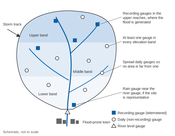
- Cover the upper catchment. WMO asks for gauges placed so that basin rainfall can be estimated for each stream gauge, usually at or near it and in the upper basin [1]. IS 4987 asks for a denser network, particularly upstream, where a catchment lies in the path of the low pressure systems that bring its rain [2].
- Sample every elevation band and the storm-facing slopes. The Arizona study chose its gauge sites with the catchment's complex topography and dominant storm track in mind, and found that a sparse but well-placed network could be accurate [5].
- Do not assume the river gauge site is representative. WMO notes that a rain gauge should be placed at the stream gauge only if it represents the general area, and not, for example, in a narrow, deep valley [1].
- Match the reporting interval to the response time. In small, steep catchments the flood peak can follow a burst of rain within tens of minutes; see time of concentration and flash floods vs river floods.
How to check an existing rain gauge network
Most districts already have gauges run by IMD, state departments or project authorities. Before adding more, check what you have.
- Density by terrain. Count gauges in each physiographic unit or elevation band and compare with the WMO and IS 4987 tables. Bands with no gauges at all are the first gaps.
- Gaps. Draw Thiessen polygons. Polygons much larger than the target area per gauge, or covering the wettest slopes, show where to add gauges.
- Statistical adequacy. Compute Cv for annual totals and for several significant storms and apply N = (Cv/ε)².
- Saturation test. A saturated network is one to which more gauges would not appreciably change the assessed rainfall. IS 4987 tests it by computing storm rainfall from all gauges, then evenly spread subsets of 80 %, 60 % and so on, and plotting the result against gauge numbers. If the estimate barely moves, the network is near saturation; if it changes rapidly, add gauges [2].
- Redundancy. IS 4987 allows closing a station whose data can be estimated accurately from neighbours by correlation, but warns against closing one before it has a stable record [2].
- Key gauges for forecasting. In the lower Mahanadi basin, Kar and co-workers chose key networks of 7 of the 14 gauges in the Kantamal sub-catchment by multi-criteria and clustering methods; the best gave a flood forecasting efficiency of 82.74 % at one-day lead time [6]. Telemetering a well-chosen subset first is a practical start.
- Recording share. Check that at least 10 % of gauges record, and that they sit where intense, short rain matters most [1, 2].
Key points
- WMO minimum densities for non-recording gauges: 250 km² per gauge in mountains, 575 km² in plains and hilly terrain, 900 km² on coasts; urban areas need a recording gauge every 10 to 20 km² [1].
- IS 4987:1994: 500 km² per gauge in plains, 250 to 400 km² at about 1 km elevation, at most 150 km² in very wet hills; minimum network 750 km² in plains, 100 to 250 km² in hills [2].
- The optimum number of rain gauges is N = (Cv/ε)², with ε usually 10 %. Use storm Cv for flood work; it is much larger than annual Cv.
- Hills need more gauges: rainfall varies over short distances and with elevation.
- At least 10 % of gauges should be recording; for flood warning, the gauges in the upper catchment should be recording and telemetered.
- Check an existing network for gaps, saturation and redundancy before adding gauges.
At ClimMaTech we start rain gauge planning from the catchments above the places that need warning, using the same density checks and statistics described here. Our weather station, VARSHAQ, is in development, and the way rainfall and river data come together for warnings is on the flood warning page.
References
- World Meteorological Organization, Guide to Hydrological Practices, Volume I: Hydrology – From Measurement to Hydrological Information, WMO-No. 168, 2008 edition, updated in 2020, section 2.4.2 and Table I.2.6, WMO, Geneva. old.wmo.int (PDF)
- Bureau of Indian Standards, Recommendations for Establishing Network of Raingauge Stations (First Revision), IS 4987:1994, BIS, New Delhi, 1994. archive.org (Public.Resource.Org, archived copy); status: BIS standards catalogue
- F. A. Huff, Sampling errors in measurement of mean precipitation, Journal of Applied Meteorology 9(1), 35–44, 1970. doi.org/10.1175/1520-0450(1970)009<0035:SEIMOM>2.0.CO;2009%3C0035:SEIMOM%3E2.0.CO;2)
- R. L. Bras, I. Rodríguez-Iturbe, Network design for the estimation of areal mean of rainfall events, Water Resources Research 12(6), 1185–1195, 1976. doi.org/10.1029/WR012i006p01185
- T. H. M. Volkmann, S. W. Lyon, H. V. Gupta, P. A. Troch, Multicriteria design of rain gauge networks for flash flood prediction in semiarid catchments with complex terrain, Water Resources Research 46, 2010WR009145, 2010. doi.org/10.1029/2010WR009145
- A. K. Kar, A. K. Lohani, N. K. Goel, G. P. Roy, Rain gauge network design for flood forecasting using multi-criteria decision analysis and clustering techniques in lower Mahanadi river basin, India, Journal of Hydrology: Regional Studies 4, 313–332, 2015. doi.org/10.1016/j.ejrh.2015.07.003
- V. Gupta, M. K. Jain, Impact of ENSO, global warming, and land surface elevation on extreme precipitation in India, Journal of Hydrologic Engineering 25(1), 05019032, 2020. doi.org/10.1061/(ASCE)HE.1943-5584.0001872HE.1943-5584.0001872)
- K. Adhikari, Y. Choden, T. Cheki, L. Gurung, T. Denka, V. Gupta, Performance evaluation of satellite precipitation estimation with ground monitoring stations over southern Himalayas in Bhutan, Acta Geophysica 68(3), 933–943, 2020. doi.org/10.1007/s11600-020-00434-z
- A. K. Mishra, P. Coulibaly, Developments in hydrometric network design: A review, Reviews of Geophysics 47, 2009. doi.org/10.1029/2007RG000243