
Time of concentration: why small catchments flood so fast
What time of concentration is, how it differs from lag time and time to peak, how to estimate it with the Kirpich formula and the NRCS velocity method, and why it sets the design storm in the rational method.

A culvert on a hill road is overtopped barely half an hour after a cloudburst begins. A city underpass fills before the rain has properly stopped. In both cases the water arrived faster than anyone expected, and the number that explains it is the time of concentration. This article explains what the term means, how it differs from lag time and time to peak, which time of concentration formula to use (Kirpich, the NRCS velocity method and the NRCS lag method), and how the answer feeds into the rational method. Two illustrative worked examples, one Himalayan hill catchment and one urban drainage area, show the arithmetic and how far the methods disagree.
What is time of concentration, and how is it different from lag time?
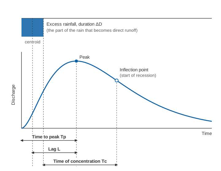
Time of concentration (Tc) is the time runoff takes to travel from the hydraulically most distant point of a catchment to its outlet. The USDA Natural Resources Conservation Service (NRCS) National Engineering Handbook adds that the hydraulically most distant point is the one with the longest travel time, not necessarily the one furthest away [1]. The Indian Roads Congress guidelines for small bridges and culverts, IRC:SP:13 (quoted here from its 2004 first revision; the second revision appeared in 2022), use the same idea: the time taken by runoff from the farthest point on the catchment boundary (the "critical point") to reach the culvert [2].
Two related terms are often confused with it:
- Lag time (L) is, in the NRCS wording, the delay between the start of runoff from a rainfall event and the runoff peak. In hydrograph analysis the NRCS defines it as the interval between the centre of mass of the excess rainfall (the part of the rain that becomes direct runoff) and the peak of the runoff [1].
- Time to peak (Tp) is the time from the start of effective rainfall to the peak discharge of a single-peaked hydrograph [3].
On the NRCS dimensionless unit hydrograph, Tc is measured from the end of excess rainfall to the point of inflection on the falling limb, where the recession begins [1]. For average natural catchments with roughly uniform runoff, NRCS uses:
L = 0.6 · Tc (L and Tc in hours)This relation comes from Mockus (1957) and Simas (1996), as reported by the handbook [1]. It is a convenience, not a law. A review of response-time methods by Gericke and Smithers notes that, depending on how lag is defined, the ratio Tc/L has been given as 1.417 or 1.67, and that a study of small catchments in Lesotho and South Africa found lag roughly equal to Tc [3]. If you are handed a "response time", always ask which of the three it is.
For more on reading the rising limb, peak and recession, see what a hydrograph tells you.
Why small, steep and paved catchments have a short Tc
Tc is a distance divided by a speed. IRC:SP:13 puts it plainly: it depends on the distance from the critical point to the structure and on the average velocity of flow, which is governed by slope, roughness and depth [2]. Three things therefore shorten it:
- Small size. A short flow path is crossed quickly.
- Steep slopes. Water on a 20 % hillside moves much faster than on a 1 % plain.
- Smooth surfaces. Roofs, roads and lined drains offer little resistance. The NRCS lists what urbanisation does: it lowers the retardance to flow, replaces slow overland flow with streets, gutters and storm sewers, and shortens overland flow lengths by getting runoff into a channel as soon as possible. Travel time generally falls [1].
The consequence for warning is direct. When rain lasts at least as long as Tc, the whole catchment contributes to the peak at once, so with a short Tc a brief, intense burst produces the full peak, soon after the burst. The flash floods vs river floods article works through what this means for lead time and sensor reporting intervals.
Tc is also not fixed. Citing Rao and Delleur (1974), the NRCS notes that lag, and hence Tc, varies from storm to storm; at Brien Run in Maryland (about 5 km²) three storms gave lags of 1.94 to 2.44 hours [1].
How to estimate time of concentration
There are two broad families of methods [3]: empirical formulas that relate Tc to a few catchment properties (length, fall, slope, land cover) by regression on measured catchments, of which Kirpich is the best known; and hydraulic methods that divide the flow path into segments and add up travel times, of which the NRCS velocity method is the standard. Where rainfall and level records exist, the response can also be measured directly, which describes your catchment rather than someone else's.
What is the Kirpich formula for time of concentration in metric units?
Kirpich published his equation in 1940 from small agricultural catchments in the United States. The NRCS describes the data set as seven rural watersheds on a farm in Tennessee with well-defined channels and steep slopes, with drainage areas of 1.25 to 112 acres (about 0.5 to 45 ha) [1]; Gericke and Smithers give average catchment slopes of 3 to 10 % [3].
IRC:SP:13 gives the form used in Indian culvert design [2]:
tc = (0.87 × L³ / H)^0.385

tc = time of concentration, hours
L  = distance from the critical point to the structure, km
H  = fall in level from the critical point to the structure, m
IRC:SP:13 credits this relation to California Culvert Practice (1944) [2], and it is algebraically the Kirpich equation. Writing the slope as S = H / (1000 L) gives the other common metric forms:
tc (hours)   = 0.0663 × L^0.77 × S^−0.385     (L in km, S in m/m)
tc (minutes) = 0.0195 × L^0.77 × S^−0.385     (L in m,  S in m/m)
The first is how Gericke and Smithers present Kirpich in SI units [3]. The check: (0.87/1000)^0.385 = 0.0663 hours, which is 3.98 minutes for L in km, and 3.98 × 1000^−0.77 = 0.0195 for L in metres.
Two cautions follow. It was calibrated on tiny farm catchments, so a 20 % Himalayan slope or a 50 km² basin is extrapolation. And it knows nothing about surface type. Gericke and Smithers report that Kirpich estimates should be multiplied by 0.4 for overland flow and 0.2 for channel flow where flow paths are lined with concrete or asphalt, and that McCuen and co-workers (1984) found the method tended to underestimate Tc in 75 % of the urbanised catchments smaller than 8 km² they tested [3].
The NRCS velocity (segment) method
The velocity method treats Tc as the sum of travel times along the hydraulically most distant flow path [1]:
Tc = Tt1 + Tt2 + … + Ttn Tt = segment length / segment velocityThe handbook uses three kinds of segment [1]:
- Sheet flow: a thin film over plane surfaces near the ridge, typically for no more than about 100 ft (30 m). Travel time comes from a simplified kinematic equation with Manning's roughness n for sheet flow (0.011 for concrete or asphalt, 0.24 for dense grass, 0.40 to 0.80 for woods), the 2-year 24-hour rainfall P2 and the land slope. Converted from the handbook's feet and inches to metres and millimetres (our conversion):
Tt (hours) = 0.091 × (n · L)^0.8 / (P2^0.5 · S^0.4)
L = sheet flow length (m), P2 = 2-year, 24-hour rainfall (mm), S = slope (m/m)- Shallow concentrated flow: flow collected in swales, rills and gullies, 0.1 to 0.5 ft (3 to 15 cm) deep. Velocity depends on slope and surface. Converted to metres per second, the handbook's equations include V = 6.20 √S for pavement and small upland gullies, 2.12 √S for short-grass pasture and 1.53 √S for woodland.
- Channel flow: where a channel is visible or surveyed. Velocity comes from Manning's equation at bankfull, V = (1/n) R^(2/3) S^(1/2) in SI units, with hydraulic radius R and channel slope S.
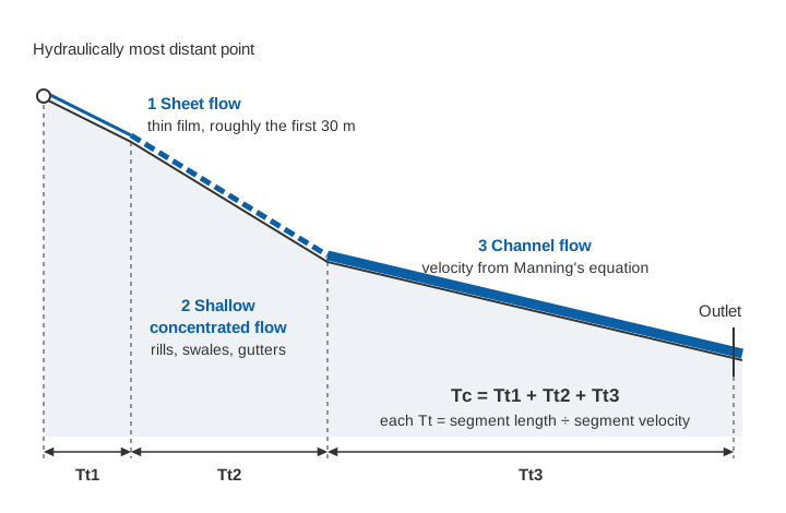
The NRCS calls the velocity method hydraulically sound and the best method for urbanising catchments, because each segment can be changed when a drain is built or a channel lined [1]. Its weak point is the inputs: Folmar and Miller (2008), cited in the handbook, found both NRCS methods tended to underestimate Tc on 52 non-urban watersheds, through lengths that ignore sinuosity, velocities that ignore pools and Manning's n set too low [1].
The NRCS watershed lag method
For catchments without detailed flow-path data, the NRCS lag equation (Mockus 1961) estimates lag from flow length, average land slope and curve number, then converts it with L = 0.6 Tc [1]. In the handbook's units:
Tc = l^0.8 × (S + 1)^0.7 / (1140 × Y^0.5)

Tc = hours, l = flow length (ft), Y = average land slope (%),
S  = 1000/CN − 10 (inches), CN = curve number (use 50 to 95)
It was developed on 24 watersheds from 1.3 acres to 9.2 square miles (up to about 24 km²) [1].
Worked example 1: a Himalayan hill catchment
The numbers are illustrative, not a real site. A stream drains 6 km² of steep, forested hillside to a road culvert. The longest flow path is 4.0 km, falling 800 m from the ridge (2,000 m) to the culvert (1,200 m), so the average slope is 800 / 4,000 = 0.20.
Kirpich (IRC:SP:13 form):
0.87 × 4.0³ / 800 = 0.0696
tc = 0.0696^0.385 = 0.358 h ≈ 21.5 minutes
NRCS velocity method, with P2 = 100 mm (assumed):
Sheet flow:   30 m, woods n = 0.40, S = 0.30
              Tt1 = 0.091 × (0.40 × 30)^0.8 / (100^0.5 × 0.30^0.4)
                  = 0.091 × 7.30 / (10 × 0.618) = 0.108 h ≈ 6.5 min
Shallow flow: 400 m, woodland, S = 0.35
              V = 1.53 × √0.35 = 0.91 m/s;  Tt2 = 400 / 0.91 = 441 s ≈ 7.3 min
Channel flow: 3,570 m, fall 651 m, S = 0.182; assumed n = 0.10, R = 0.5 m
              V = (1/0.10) × 0.5^(2/3) × 0.182^0.5 = 10 × 0.630 × 0.427 = 2.69 m/s
              Tt3 = 3,570 / 2.69 = 1,327 s ≈ 22.1 min
Tc = 6.5 + 7.3 + 22.1 ≈ 36 minutes
NRCS lag method, with CN = 70 and average land slope Y = 40 % (both assumed):
l = 4,000 m = 13,123 ft;   S = 1000/70 − 10 = 4.29
Tc = 13,123^0.8 × 5.29^0.7 / (1140 × 40^0.5) = 1,970 × 3.21 / 7,210 = 0.88 h ≈ 53 minutes
Three accepted methods give 21.5, 36 and 53 minutes on the same catchment, a factor of 2.5. That spread is normal: Grimaldi and co-workers compared Tc approaches on four small basins and found predictions differing by up to 500 % [4]. The Kirpich result is also an extrapolation (a 20 % slope, twice the upper end of the 3 to 10 % slopes it was calibrated on), and the channel time hinges on Manning's n, which is least certain in steep boulder channels. With the velocity-method Tc, L = 0.6 × 36 ≈ 22 minutes: the peak could follow the centre of the burst by about twenty minutes.
Worked example 2: an urban drainage area, before and after paving
Again illustrative. A 1.2 km² area drains along a 1.68 km path: 30 m of sheet flow, 150 m of shallow concentrated flow (both at S = 0.01), then 1,500 m of channel at S = 0.004, a total fall of 7.8 m. P2 = 100 mm.
| Segment | Before development | After development |
|---|---|---|
| Sheet flow, 30 m | Dense grass, n = 0.24: 16.8 min | Asphalt, n = 0.011: 1.4 min |
| Shallow flow, 150 m | Pasture, V = 2.12 × √0.01 = 0.21 m/s: 11.8 min | Pavement, V = 6.20 × √0.01 = 0.62 m/s: 4.0 min |
| Channel, 1,500 m | Natural drain, assumed V = 0.6 m/s: 41.7 min | Lined drain, assumed V = 1.5 m/s: 16.7 min |
| Tc | 70 min | 22 min |
Paving and lining cut Tc to less than a third. Kirpich, using only L and H, cannot see this:
0.87 × 1.68³ / 7.8 = 0.529;  tc = 0.529^0.385 = 0.78 h ≈ 47 min
with the paved-surface factors: 0.4 × 47 ≈ 19 min;  0.2 × 47 ≈ 9 min
So for the developed state the estimates range from 9 to 47 minutes depending on the method and factor chosen.
Try the Kirpich formula
Enter the length of the flow path and the fall along it. The calculator applies the IRC:SP:13 form, shows the slope and the equivalent lag, and warns when you are outside the conditions Kirpich was calibrated on.
Illustrative calculator. Kirpich is an empirical formula from small farm catchments; use it for orders of magnitude and compare it with a segment-by-segment estimate.
Which time of concentration do you use in the rational method?
You use Tc as the duration of the design storm. IRC:SP:13 explains why: shorter bursts are more intense, so it seems safer to design for a very short duration, but a burst shorter than Tc ends before water from the distant parts of the catchment reaches the structure. Only the intensity for a duration equal to Tc needs to be considered [2].
The rational method then gives the peak discharge:
Q = C · i · A / 3.6

Q = peak discharge (m³/s), C = runoff coefficient (0 to 1),
i = rainfall intensity for duration Tc (mm/h), A = catchment area (km²)
The 3.6 is a unit conversion: 1 mm/h over 1 km² is 0.001 m × 1,000,000 m² / 3,600 s = 0.278 m³/s. IRC:SP:13 writes the same formula as Q = 0.028 P A Ic, with A in hectares, Ic in cm/h and P its runoff coefficient; its table of maximum values gives, for example, 0.90 for steep bare rock and city pavements, 0.80 for steep wooded rock and 0.30 for largely cultivated loam [2].
For the intensity, IRC:SP:13 starts from the region's one-hour rainfall I₀ and adjusts it to the catchment's Tc [2]:
Ic = I₀ × 2 / (tc + 1) (tc in hours)IRC:SP:13 also applies a factor f, read from a curve, that lowers the mean intensity as catchment area grows; we leave it out to keep the arithmetic visible.
Hill catchment (A = 6 km², C = 0.6, I₀ = 5 cm, all assumed). With 0.6 × 6 / 3.6 = 1.0, Q in m³/s equals i in mm/h:
| Tc used | Ic = 2 × 5 / (tc + 1) | Q |
|---|---|---|
| Kirpich, 0.36 h | 7.36 cm/h = 73.6 mm/h | 74 m³/s |
| Velocity method, 0.60 h | 6.25 cm/h = 62.5 mm/h | 63 m³/s |
| Lag method, 0.88 h | 5.33 cm/h = 53.3 mm/h | 53 m³/s |
The Tc choice alone moves the design peak by about 40 %. Gericke and Smithers note that underestimating Tc overestimates the peak and the reverse, and cite estimates that up to 75 % of the error in peak discharge can come from the time parameter [3].
Urban area (A = 1.2 km², I₀ = 5 cm). Before development: Tc = 70 min (1.17 h), Ic = 10 / 2.17 = 4.61 cm/h = 46.1 mm/h, C = 0.30, so Q = 0.30 × 46.1 × 1.2 / 3.6 = 4.6 m³/s. After: Tc = 22 min (0.37 h), Ic = 10 / 1.37 = 7.31 cm/h = 73.1 mm/h, C = 0.90, so Q = 0.90 × 73.1 × 1.2 / 3.6 = 21.9 m³/s. The peak grows almost fivefold: a factor of 3 from the runoff coefficient and about 1.6 from the shorter Tc. Where local intensity–duration–frequency data exist, use them; the one-hour relation only keeps both examples on the same basis.
Practical advice
- Compute at least two methods and state the inputs. If they disagree by a factor of two, that is the honest uncertainty. Gericke and Smithers conclude that empirical methods should not be applied beyond the regions where they were developed without local correction factors [3].
- Measure it when you can. A rain gauge in the catchment and a water level recorder at the outlet, logging at short intervals, give observed lag times from real storms.
Key points
- Tc runs from the hydraulically most distant point to the outlet; lag from the centroid of excess rain to the peak; time to peak from the start of excess rain to the peak.
- NRCS uses L ≈ 0.6 Tc for average natural catchments; other definitions give other ratios.
- Kirpich (IRC:SP:13 form): tc (h) = (0.87 L³ / H)^0.385, L in km, H in m, calibrated on small farm catchments.
- The velocity method adds sheet, shallow concentrated and channel flow times and suits urban and changing catchments.
- Methods often disagree by a factor of two or more, and because Tc sets the rational-method storm duration, the disagreement reaches the design peak.
- Small, steep and paved catchments have short Tc: brief bursts produce the full peak and leave little warning time.
At ClimMaTech we look at catchment response time first when planning where to place rain gauges and water-level sensors, because it decides how close to the source the measurements must be and how often they must report. Our approach for rivers and hill streams is on the flood warning page, and for drains, underpasses and low-lying streets on the urban flooding page.
References
- United States Department of Agriculture, Natural Resources Conservation Service, National Engineering Handbook, Part 630 Hydrology, Chapter 15: Time of Concentration, 210-VI-NEH, USDA NRCS, 2010. directives.nrcs.usda.gov (PDF)
- Indian Roads Congress, Guidelines for the Design of Small Bridges and Culverts, IRC:SP:13-2022 (second revision), IRC, New Delhi, 2022 irc.nic.in; text quoted from IRC:SP:13-2004 (first revision), Article 4 (empirical and rational formulae for peak run-off), IRC, New Delhi, 2004. law.resource.org (PDF, archived copy)
- O. J. Gericke, J. C. Smithers, Review of methods used to estimate catchment response time for the purpose of peak discharge estimation, Hydrological Sciences Journal 59(11), 1935–1971, 2014. doi.org/10.1080/02626667.2013.866712
- S. Grimaldi, A. Petroselli, F. Tauro, M. Porfiri, Time of concentration: a paradox in modern hydrology, Hydrological Sciences Journal 57(2), 217–228, 2012. doi.org/10.1080/02626667.2011.644244