
Intensity-duration-frequency (IDF) curves in hydrology
What an IDF curve shows, how it is built from annual maximum rainfall and Gumbel frequency analysis, what the IDF formula means, and how to read a design intensity for drains and culverts.

An engineer sizing a storm drain or a culvert first needs to know how hard it can rain, for how long, and how often. The IDF curve in hydrology answers that: an intensity-duration-frequency (IDF) curve gives the average rainfall intensity to expect over a given duration for a chosen return period, at one place. This article explains what the curve shows, how it is built from annual maximum rainfall with Gumbel frequency analysis, what the IDF formula means, and how to read a design intensity for the rational method, with an illustrative worked example and a calculator.
What is an IDF curve?
An IDF curve is a graph of rainfall intensity (depth per unit time, usually mm/h) against duration (minutes or hours), drawn as one curve for each return period. The WMO Guide to Hydrological Practices describes IDF relationships as the usual engineering summary of point-rainfall frequency analysis, typically for durations from five minutes to two days and return periods from two to one hundred years [1].
Three ideas sit in the name:
- Intensity (i): the average rate of rain over the duration, so a 30-minute depth of 50 mm is an intensity of 100 mm/h.
- Duration (t): the window over which rain is averaged, usually a window inside a storm rather than the whole storm.
- Frequency: expressed as a return period T, the average number of years within which the intensity is expected to be equalled or exceeded once. The return period is the reciprocal of the annual exceedance probability [1].
Every IDF curve falls from left to right, because short windows capture the most intense part of a storm, and the curves stack upwards with return period.
Return period is a probability, not a timetable
A "25-year" intensity has a 1/25 = 4 % chance of being equalled or exceeded in any one year; it can happen twice in a decade. The chance of at least one exceedance in N years follows the Bernoulli relation in WMO-No. 168 [1]:
Rn = 1 − (1 − 1/T)^N

T = 25 years, N = 25 years:   Rn = 1 − 0.96^25 = 1 − 0.360 = 0.64
T = 100 years, N = 50 years:  Rn = 1 − 0.99^50 = 1 − 0.605 = 0.39
A drain designed for the 25-year intensity therefore has about a 64 % chance of being exceeded at least once in 25 years of service: the risk the chosen return period accepts.
How is an IDF curve built?
NOAA Atlas 14, the US precipitation-frequency atlas, documents each step [2], and IMD's IDF study follows the same outline [3].
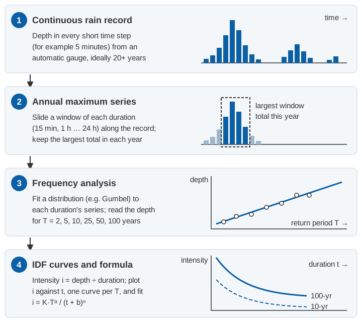
1. A continuous rain record at short time steps for many years, from a recording or automatic gauge. Daily totals cannot tell you how much fell in the worst half hour.
2. An annual maximum series for each duration. For each duration (say 15 minutes to 24 hours) slide a window of that length along the record and keep the largest total in each year. The WMO Guide notes that the annual maximum series is the most common choice and that, for return periods above about ten years, results differ little from a partial duration (peaks-over-threshold) series [1].
If totals exist only for fixed clock hours or observation days, the true maximum is usually missed because the burst straddles two intervals. IMD's IDF study multiplies clock-hour and observation-day totals by 1.15 to estimate the maximum over any 60 minutes or 24 hours [3]; NOAA Atlas 14 uses 1.09 for 1-hour and 1.12 for 1-day data [2].
3. Frequency analysis. Fit a distribution to each duration's series and read off the depth for each return period. Of the distributions commonly applied to annual maxima, the WMO Guide notes that the generalised extreme value (GEV) distribution and its special case, the Gumbel, dominate rainfall work [1]. IMD's study of 120 self-recording rain gauge (SRRG) stations used the Gumbel distribution [3]; NOAA Atlas 14 used regional L-moments and adopted the GEV in its south-eastern US volume [2].
4. Intensities and curves. Divide each depth by its duration, plot intensity against duration for each return period, and fit an equation if you want one.
Gumbel frequency analysis: the frequency-factor method
The Gumbel (extreme value type I, EV1) distribution has the cumulative distribution F(x) = exp{−exp[−(x − ξ)/α]}, with location ξ and scale α. Its mean is ξ + 0.5772α and its variance is π²α²/6 [1]. Matching these to the sample mean x̄ and standard deviation s (the method of moments, the simplest of the estimation methods the Guide describes [1]) gives a compact rule:
x_T = x̄ + K_T · s

K_T = −(√6 / π) · [0.5772 + ln( ln( T / (T − 1) ) )]

x_T = depth with return period T, x̄ = mean of the annual maxima,
s = sample standard deviation, √6 / π = 0.7797
K_T is the frequency factor: how many standard deviations above the mean the T-year value lies. It depends only on T:
| T (years) | ln(T/(T−1)) | ln of that | K_T |
|---|---|---|---|
| 2 | 0.69315 | −0.3665 | −0.164 |
| 5 | 0.22314 | −1.4999 | 0.719 |
| 10 | 0.10536 | −2.2504 | 1.305 |
| 25 | 0.04082 | −3.1985 | 2.044 |
| 50 | 0.02020 | −3.9019 | 2.592 |
| 100 | 0.01005 | −4.6001 | 3.137 |
For example, at T = 10: 0.5772 − 2.2504 = −1.6732, and −0.7797 × (−1.6732) = 1.305.
Two cautions from the WMO Guide: the Gumbel distribution has been found to underestimate extreme rainfall, with three-parameter distributions such as the GEV often fitting better; and L-moments are less biased than ordinary moments for short records [1]. The frequency-factor method is a clear way to learn the procedure, not the only defensible one.
An intensity-duration-frequency curve example
The numbers below are illustrative, not records from a real station. Suppose an automatic gauge has 20 years of 5-minute data, and the largest 60-minute total in each year is (mm):
| Years 1–10 | 38 | 61 | 45 | 72 | 50 | 41 | 83 | 56 | 47 | 35 |
|---|---|---|---|---|---|---|---|---|---|---|
| Years 11–20 | 66 | 52 | 44 | 90 | 49 | 58 | 40 | 63 | 54 | 46 |
Step 1: mean and standard deviation.
Sum = 1,090 mm;  n = 20;  x̄ = 1,090 / 20 = 54.5 mm
Σ(x − x̄)² = 4,071;  s = √(4,071 / 19) = √214.3 = 14.64 mm
Step 2: depths for each return period, x_T = 54.5 + K_T × 14.64:
T = 2:    54.5 − 0.164 × 14.64 = 52.1 mm
T = 10:   54.5 + 1.305 × 14.64 = 73.6 mm
T = 25:   54.5 + 2.044 × 14.64 = 84.4 mm
T = 50:   54.5 + 2.592 × 14.64 = 92.4 mm
T = 100:  54.5 + 3.137 × 14.64 = 100.4 mm
For 60 minutes, depth in mm equals intensity in mm/h. With 20 years of record, the 50- and 100-year values are extrapolations; the WMO Guide notes that frequency values are generally not published for return periods longer than roughly twice the record [1].
Step 3: repeat for every duration, using each duration's (illustrative) annual maxima, and convert depth to intensity with i = depth × 60 / t (t in minutes).
| Duration | Mean, s of annual maxima (mm) | i, T = 2 | i, T = 10 | i, T = 25 | i, T = 100 (mm/h) |
|---|---|---|---|---|---|
| 15 min | 24.0, 7.0 | 91.4 | 132.5 | 153.2 | 183.8 |
| 30 min | 36.0, 10.5 | 68.6 | 99.4 | 114.9 | 137.9 |
| 1 h | 54.5, 14.6 | 52.1 | 73.6 | 84.4 | 100.4 |
| 3 h | 74.0, 24.0 | 23.4 | 35.1 | 41.0 | 49.8 |
| 6 h | 92.0, 30.0 | 14.5 | 21.9 | 25.6 | 31.0 |
| 24 h | 135.0, 46.0 | 5.3 | 8.1 | 9.5 | 11.6 |
Check one cell: for 15 minutes and T = 25, x = 24.0 + 2.044 × 7.0 = 38.3 mm, and i = 38.3 × 60 / 15 = 153.2 mm/h.
What is the IDF curve formula?
A formula is easier to use than a table. The WMO Guide lists typical empirical forms such as i = a/(t + b) and i = aT/(t + b) [1]. A form used in Indian station studies, traced by Anand and co-authors to Bernard (1932), combines return period and duration [4]:
i = K · T^a / (t + b)^n

i = average intensity over duration t (units as fitted, e.g. mm/h)
T = return period (years)
t = duration (units as fitted, e.g. minutes or hours)
K, a, b, n = constants fitted for one station or region
T^a lifts the curve as the return period grows; b and n set how fast intensity falls with duration. The constants only hold in the units they were fitted in: for Washim district in Vidarbha, Maharashtra, Anand and co-authors obtained K = 2.754, a = 0.216, b = 0.32 and n = 0.614 with i in cm/h and t in hours [4]. Used with minutes, the same numbers give nonsense.
Fitting all the intensities computed in the worked example (eight durations from 15 minutes to 24 hours and six return periods from 2 to 100 years; the table shows a subset) by least squares on the logarithms of intensity gives:
i (mm/h) = 1181 · T^0.183 / (t + 20)^0.748 t in minutesThe fitted formula reproduces those 48 intensities with a root-mean-square error of about 4 % and a worst case of about 9 %. Kothyari and Garde (1992) went further: from 80 Indian rain-gauge stations, and on the premise that the convective cells behind short rainfalls have similar properties in different regions, they developed a general IDF relationship for India [5].
How to read a design intensity, and link it to the rational method
Reading an IDF curve takes two decisions: the return period, a design-standard choice, and the duration, which comes from the catchment. In the rational method the duration equals the time of concentration (tc), the travel time from the most distant point to the outlet; the WMO Guide adds that return periods of 2 to 10 years are typical for minor drainage systems [1]. IRC:SP:13 gives the reason: a shorter burst ends before water from the far parts of the catchment arrives [6].
The rational method then gives the peak flow [1]:
Q = 0.278 · C · i · A

Q = peak discharge (m³/s), C = runoff coefficient,
i = intensity for duration tc (mm/h), A = catchment area (km²)
Example (illustrative). The hill catchment in our time-of-concentration article had an estimated tc of 36 minutes by the velocity method, an area of 6 km² and an assumed C of 0.6. From the illustrative curve, for T = 25 years:
i = 1181 × 25^0.183 / (36 + 20)^0.748 = 1181 × 1.802 / 20.31 = 104.8 mm/h
Q = 0.278 × 0.6 × 104.8 × 6 = 104.9 m³/s
For T = 10 years, i = 88.6 mm/h and Q = 88.7 m³/s. An IDF curve describes point rainfall; IRC:SP:13 and the CWC flood estimation reports reduce it for larger areas [6, 7], a step left out here.
The Indian picture: where IDF data come from
What IMD, CWC and IRC provide
- IMD. Das, Srivastava and Yadav used SRRG data for 1969–2013 from 120 stations (83 with more than 30 years of data, 37 with 20 to 29) to draw isopluvial maps for 1 to 24 hours and 2 to 100 years, and IDF curves for 28 stations [3].
- CWC. The regional flood estimation reports are joint work of CWC, IMD, RDSO and the then Ministry of Surface Transport. The Western Himalayas (zone 7) report contains an IMD rainfall study with 24-hour isopluvial maps for 25, 50 and 100 years and ratios to convert 24-hour rainfall to shorter durations [7].
- IRC:SP:13. The guidelines for small bridges and culverts (second revision 2022; the details here are from the 2004 first revision) characterise a region by its "one-hour rainfall" I₀. They relate the mean intensity i over t hours inside a storm to the storm's mean intensity I over D hours by i/I = (D + 1)/(t + 1), which leads to the critical intensity Ic = I₀ × 2/(tc + 1). The 2004 edition reproduces IMD's chart of the heaviest one-hour rainfall at Indian stations, with values up to 1966 [6].
Why short-duration data are scarce
Kothyari and Garde noted in 1992 that little information was available on Indian rainfall intensities, particularly for short durations [5]. The CWC Western Himalayas report shows why: it had daily data from 202 ordinary rain gauges but hourly data from only 20 SRRG stations, just 9 of them with 8 to 13 years of record. Its short-duration ratios, averaged over those 9 stations, were recommended for the whole zone [7]:
| Duration (h) | 1 | 3 | 6 | 9 | 12 | 15 | 18 | 24 |
|---|---|---|---|---|---|---|---|---|
| 10-year t-hour ÷ 10-year 24-hour rainfall | 0.425 | 0.600 | 0.725 | 0.790 | 0.845 | 0.895 | 0.935 | 1.000 |
IMD's 2022 study makes the same point: a lack of hourly records makes IDF curves less reliable [3]. Below an hour, the WMO Guide quotes US-derived average ratios of 5-, 10-, 15- and 30-minute to 60-minute rainfall of 0.29, 0.45, 0.57 and 0.79, and warns that they can be too low where rain is mostly from thunderstorms and too high in orographic regions [1]. Ratios are a fallback, not a substitute for local data.
Sub-daily data from automatic gauges
Automatic rain gauges and weather stations log rainfall at fixed intervals, so sliding-window maxima can be extracted for any duration down to the logging interval. IMD's network grew from 1,350 automatic rain gauges in 2014 to 1,382 in 2023, and its automatic weather stations from 675 to 1,008 [8]. The catch is time: a curve built on a few years of sub-daily data should be checked against regional studies. Where gauges are sparse, regional frequency analysis pools stations that behave alike; in our study of north-east India, regions defined by fuzzy clustering of IMD station data passed L-moment homogeneity tests for regional frequency analysis [9]. Gauge errors also propagate into the maxima (see the tipping-bucket rain gauge article).
Climate change and nonstationarity
Classical IDF analysis assumes the annual maxima are independent and identically distributed: a stationary climate [1]. NOAA Atlas 14 ran trend tests before accepting this for its project area [2]. In our study of extreme precipitation indices across India, total wet-day rainfall showed decreasing trends over a larger part of the country, yet most extreme precipitation indices showed increasing trends [10]. Ali and Mishra found that at most of the Indian urban stations they studied, rainfall extremes rise strongly with dew-point temperature, and that daily design storms estimated under a nonstationary assumption were higher than stationary ones [11].
In practice: state the period of record behind any IDF curve, test the annual maxima for trend before fitting, and revisit curves as records lengthen.
Try the IDF formula
Choose a set of constants (this article's illustrative curve, the published Washim equation or your own), then set the return period and duration.
Illustrative calculator. The default constants come from the illustrative worked example; published constants apply only to their own station, units and period of record.
Key points
- An IDF curve gives the average rainfall intensity over a duration for a chosen return period at one place.
- It is built from each duration's annual maximum series, extracted from sub-daily records, followed by frequency analysis.
- Gumbel frequency-factor method: x_T = x̄ + K_T s, with K_T = −0.7797 [0.5772 + ln ln(T/(T − 1))].
- The constants of i = K T^a/(t + b)^n hold only in their own units and place.
- In the rational method the design duration equals the time of concentration; the return period carries a known risk of exceedance.
- Indian short-duration records are scarce; IMD and CWC regional studies fill gaps while automatic gauges build the sub-daily record.
At ClimMaTech we work with sub-daily rainfall because it is the record behind IDF curves, drain design and flash-flood warning in small catchments. Our approach for drains, underpasses and low-lying streets is on the urban flooding page, and VARSHAQ, our weather station, is in development.
References
- World Meteorological Organization, Guide to Hydrological Practices, Volume II: Management of Water Resources and Application of Hydrological Practices, WMO-No. 168, sixth edition, sections 4.2.5.2, 4.7.3.3.1, 5.2, 5.3 and 5.7, WMO, Geneva, 2009. old.wmo.int (PDF)
- S. Perica et al., NOAA Atlas 14, Precipitation-Frequency Atlas of the United States, Volume 9 Version 2.0: Southeastern States, sections 3.2 and 4.3 to 4.6, NOAA National Weather Service, Silver Spring, 2013. weather.gov (PDF)
- A. K. Das, P. Srivastava, B. P. Yadav, Isopluvial analysis and Intensity Duration Frequency (IDF) curves for different cities in India, MAUSAM 73(4), 887–898, 2022. doi.org/10.54302/mausam.v73i4.3530
- S. Anand, P. Kumar, M. Kumar, Development of rainfall intensity-duration-frequency relationships and nomographs for selected stations in Maharashtra, India, MAUSAM 74(3), 707–716, 2023. doi.org/10.54302/mausam.v74i3.6302
- U. C. Kothyari, R. J. Garde, Rainfall intensity-duration-frequency formula for India, Journal of Hydraulic Engineering 118(2), 323–336, 1992. doi.org/10.1061/(ASCE)0733-9429(1992)118:2(323)0733-9429(1992)118:2(323))
- Indian Roads Congress, Guidelines for the Design of Small Bridges and Culverts, IRC:SP:13-2022 (second revision), IRC, New Delhi, 2022 irc.nic.in; text quoted from IRC:SP:13-2004 (first revision), Article 4.7 and Appendix A, IRC, New Delhi, 2004. law.resource.org (PDF, archived copy)
- Central Water Commission, Flood Estimation Report for Western Himalayas – Zone 7, Design Office Report WH/22/1994, Part IV (rainfall studies), a joint work of CWC, RDSO, IMD and the Ministry of Surface Transport, New Delhi, 1994. cwc.gov.in (PDF)
- India Meteorological Department, Recent achievements of IMD in the last decade (2014–2023), chapter 4 of 150 Years of Service to the Nation, IMD, New Delhi, 2024. mausam.imd.gov.in (PDF)
- M. K. Goyal, V. Gupta, Identification of homogeneous rainfall regimes in northeast region of India using fuzzy cluster analysis, Water Resources Management 28(13), 4491–4511, 2014. doi.org/10.1007/s11269-014-0699-7
- V. Gupta, M. K. Jain, Impact of ENSO, global warming, and land surface elevation on extreme precipitation in India, Journal of Hydrologic Engineering 25(1), 05019032, 2020. doi.org/10.1061/(ASCE)HE.1943-5584.0001872HE.1943-5584.0001872)
- H. Ali, V. Mishra, Contrasting response of rainfall extremes to increase in surface air and dewpoint temperatures at urban locations in India, Scientific Reports 7, 1228, 2017. doi.org/10.1038/s41598-017-01306-1