Surface velocity coefficient: where 0.85 comes from

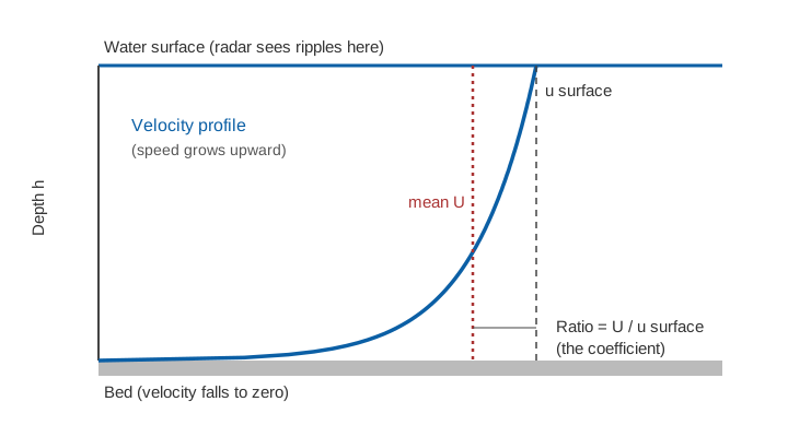
A radar, a camera or a floating twig can tell you how fast the surface of a river is moving. Discharge needs the average velocity over the whole cross-section, and that is always lower, because the water slows towards the bed. Surface velocity measurement therefore ends with a multiplication: the surface velocity is scaled by a surface velocity coefficient, usually written α (alpha), and the value most often used is 0.85. This article explains where that number comes from, what the field evidence says about it, and why it is the largest single judgement in non-contact gauging.

What is the surface velocity coefficient?

The surface velocity coefficient is the ratio of the depth-averaged velocity to the velocity at the water surface, α = U / u_s. It is also called the velocity coefficient, velocity index or alpha coefficient [6]. It is the number that turns what a sensor sees into what the discharge equation needs:

Q = A × U = A × α × u_s

Q   = discharge (m³/s)
A   = flow area of the cross-section (m²), from level and surveyed shape
U   = mean velocity over the cross-section (m/s)
u_s = surface velocity (m/s)
α   = surface velocity coefficient (dimensionless)

How does a surface velocity radar see the surface?

A surface velocity radar (SVR) measures the Doppler shift of microwaves scattered by small ripples on the water surface, a process called Bragg scattering [3]. We explain the physics in surface velocity radar: how Doppler measures river flow. The important point here is that the instrument reports the speed of the top skin of water and of the ripples riding on it. It reports nothing about the water below. To estimate the discharge, someone has to supply the shape of the velocity profile beneath.

Where does 0.85 come from?

The value 0.85 comes from two places: an engineering habit in the field and a simple mathematical profile that happens to agree with it.

Field practice: the USGS and WMO manuals

The classic reference is Measurement and Computation of Streamflow by Rantz and colleagues at the US Geological Survey (1982). It describes an optical current meter, a stroboscopic instrument that measures the speed of the water surface by eye, and says its surface velocity "must be corrected by an appropriate coefficient to obtain the mean velocity in the vertical". The precise coefficient, it adds, "is, of course, unique to the particular stream and to the location of the vertical in the stream cross section", but "for natural channels a coefficient of 0.85 has been used" and 0.90 for concrete-lined channels [1]. Elsewhere in the same volume, a coefficient of 0.85 or 0.86 is prescribed for the surface-velocity method in a natural channel, 0.90 in a smooth artificial one, and 0.85 for converting the speed of a surface float to the mean velocity in the vertical [1].

The WMO Manual on Stream Gauging (WMO-No. 1044, 2010) repeats the guidance: 0.85 for natural channels, and 0.90 for concrete-lined channels, where it will not introduce errors of more than ±5 per cent [2]. So 0.85 is a convention built from decades of comparisons with current-meter gaugings: a sensible average, not a law of nature.

The profile argument

A river's velocity profile rises from zero at the bed to a maximum near the surface. Suppose the velocity at height z above the bed follows a power law, u = u_s × (z/h)^(1/m), where h is the depth. Averaging over the depth gives:

U / u_s = 1 / (1 + 1/m) = m / (m + 1)

m = 6:   U / u_s = 6/7 = 0.857
m = 7:   U / u_s = 7/8 = 0.875

Exponents between 1/6 and 1/7 are the usual choices. The 1/6 exponent reproduces the figure of 0.857 that reviews describe as the usual "default value" [6]; the classic 1/7 exponent gives 0.875. The logarithmic law gives a different route to nearly the same number. In a log profile, u = (u/κ) ln(z/z₀), where u is the shear velocity (a measure of bed friction), κ ≈ 0.41 is von Kármán's constant and z₀ is the height at which the extrapolated velocity falls to zero, set by the roughness of the bed. Integrating over the depth and dividing by the surface value gives:

α = 1 − 1 / ln(h / z0)      (log-law profile, derived by integrating u over the depth)

So the coefficient is not fixed: it depends on relative roughness, the ratio of bed roughness to depth. The rougher the bed relative to the depth, the lower α becomes.

The curve reaches 0.85 at an h/z₀ of about 800, and shows why shallow flow over a coarse bed gives lower values and deep flow over a smooth bed higher ones. This is only a model; the next section tests it.

What do field measurements show?

Measurements agree with the idea but show real scatter.

• Radar trials on the San Joaquin and Cowlitz rivers (USA). Costa and co-authors, using radars, found that log-shaped velocity profiles held over a wide range of flows, and that "mean velocity is approximately 0.85 times measured surface velocity". The radar discharges were within a few percent of the gauging-station values, and within 5 % during a flood, although early readings at the San Joaquin were more than 20 % higher than the independent measurements [3].
• 3,611 current-meter gaugings at 176 river sites (France). Hauet and co-authors fitted log and power laws and also used the measured surface velocity. The mean α was about 0.8, with 5th and 95th percentiles near 0.7 and 0.9. α rose with hydraulic radius (roughly, with depth), but a clear link with bed roughness was not found. Natural rivers averaged 0.8 and artificial concrete channels 0.9 [5].
• Portable radars at several field sites. Welber and co-authors (2016) found that α = 0.85 is "a valid default value", but recommend site-specific calibration "to avoid underestimation of discharge in very smooth channels (relative roughness ∼ 0.001) and overestimation in very rough channels (relative roughness > 0.05)". Section-averaged coefficients varied less than those computed on single verticals, especially in channels with high relative roughness. With theoretical or calibrated values, discharge was within 10 % for low and intermediate roughness [4].
• A review of methods. Biggs and co-authors (2023) compare approaches for estimating α: reference discharge and surface velocity, extrapolated ADCP profiles, log-law and power-law fits, site characteristics and default values. They conclude that a better-chosen α "could provide a substantial accuracy improvement" over using 0.857 everywhere, and name surface wind and the velocity dip (where the maximum velocity lies below the surface) among the unresolved challenges [6].

Note the pattern. For natural channels, the default sits in the middle of the observed range. For artificial channels, it is too low. For rough, shallow mountain streams, it can be too high.

Why does the coefficient vary?

Four things move α away from 0.85:

1. Bed roughness and depth. As the log-law relation above shows, deeper or smoother flow gives a higher α. The French sample found α rising with hydraulic radius [5].
2. Stage. Depth changes with stage, so α is not constant at a site; a "stage to alpha rating curve" is one remedy [6].
3. Position across the section. Near the banks, α is lower and the velocities are less certain. Welber and co-authors found larger uncertainties close to the banks [4].
4. Wind and velocity dip. A wind blowing against the flow slows the surface skin, while a wind with the flow speeds it. Neither says anything about the water below, which is why both are listed as open problems [6].

Shallow, boulder-bed Himalayan streams have high relative roughness, so the default needs checking there; see river monitoring in hill and Himalayan catchments.

Worked example: what a coefficient error does to discharge

Because the coefficient multiplies the whole discharge, an error in α passes straight through. Take an illustrative section with a flow area of 40 m² and a section-representative surface velocity of 1.8 m/s:

α = 0.85:   Q = 40 × 0.85 × 1.8 = 61.2 m³/s
α = 0.80:   Q = 40 × 0.80 × 1.8 = 57.6 m³/s   (−5.9 %)
α = 0.90:   Q = 40 × 0.90 × 1.8 = 64.8 m³/s   (+5.9 %)

A 0.05 error in α is a 5.9 % error in discharge, before adding the uncertainty of the level measurement, the section survey and the velocity itself. That is why calibration matters when the answer feeds water accounting or a rating curve; see rating curves and their uncertainty.

How is the coefficient calibrated?

The reviews agree on a hierarchy [4][6]:

• Best: site-specific calibration against reference discharges, from current-meter gaugings or an acoustic Doppler profiler (ADCP) at different stages. The ratio of reference discharge to surface-velocity discharge gives α for that section. See the velocity-area method for the reference measurement.
• Next: profile-based estimates from a log or power law fitted to an ADCP or current-meter profile, then estimates from site characteristics.
• Last resort: the default. The default is a sensible starting point for natural channels with low to intermediate roughness, and is not to be trusted at the extremes [4].

A different route replaces the fixed coefficient altogether. The probability concept computes mean velocity and discharge from a single surface velocity and the cross-sectional area, and was tested with radars at 10 US Geological Survey streamgages, where the results were highly correlated with conventional methods [7].

Key points

• Surface velocity measurement sees only the top of the flow. Discharge needs the mean velocity, so a coefficient α = U / u_s is applied.
• The value 0.85 comes from USGS and WMO field practice (0.85 to 0.86 for natural channels, 0.90 for smooth artificial ones) and agrees with a 1/6 power-law profile, which gives 6/7 = 0.857 [1][2][6].
• Theory and data both show that α depends on depth and roughness, and that it varies with stage and position across the section [4][5][6].
• A 0.05 change in α changes discharge by about 6 %, so the default should be checked by gaugings wherever the discharge matters.
• Radar discharge within about 10 % has been reported where the coefficient was calibrated or theoretically derived and the roughness was low to intermediate [4].

Where ClimMaTech fits

PRAVAAH is ClimMaTech's non-contact discharge sensor: an AWLR (Automatic Water Level Recorder) and a Surface Velocity Radar (SVR) in one unit, measuring level and surface velocity without touching the water. The questions in this article, how the surface relates to the mean and how to check it against gaugings, apply to any non-contact discharge measurement.

References

1. S. E. Rantz and others, Measurement and Computation of Streamflow: Volume 1. Measurement of Stage and Discharge, U.S. Geological Survey Water-Supply Paper 2175, 1982 (optical current meter p. 92; surface-velocity method pp. 137–138; surface floats p. 262). pubs.usgs.gov
2. World Meteorological Organization, Manual on Stream Gauging, Volume I: Fieldwork, WMO-No. 1044, 2010, chapter 5. old.wmo.int
3. J. E. Costa, R. T. Cheng, F. P. Haeni, N. Melcher, K. R. Spicer, E. Hayes, W. Plant, K. Hayes, C. Teague, D. Barrick, Use of radars to monitor stream discharge by noncontact methods, Water Resources Research 42(7), 2006. doi:10.1029/2005WR004430
4. M. Welber, J. Le Coz, J. B. Laronne, G. Zolezzi, D. Zamler, G. Dramais, A. Hauet, M. Salvaro, Field assessment of noncontact stream gauging using portable surface velocity radars (SVR), Water Resources Research 52(2), 1108–1126, 2016. doi:10.1002/2015WR017906
5. A. Hauet, P. Morlot, C. Daubagnan, Velocity profile and depth-averaged to surface velocity in natural streams: a review over a large sample of rivers, E3S Web of Conferences 40, 06015 (River Flow 2018), 2018. doi:10.1051/e3sconf/20184006015
6. H. Biggs, G. Smart, M. Doyle, N. Eickelberg, J. Aberle, M. Randall, M. Detert, Surface velocity to depth-averaged velocity: a review of methods to estimate alpha and remaining challenges, Water 15(21), 3711, 2023. doi:10.3390/w15213711
7. J. W. Fulton and others, Near-field remote sensing of surface velocity and river discharge using radars and the probability concept at 10 U.S. Geological Survey streamgages, Remote Sensing 12(8), 1296, 2020. doi:10.3390/rs12081296