
What a hydrograph tells you: reading a flood after it has passed
How the rising limb, peak, recession and baseflow of a flood hydrograph describe a catchment, how to measure lag time and separate baseflow, and why the rising limb is the part that matters for warnings.

When a flood has passed, the river is back within its banks and the damage is being counted, the most useful record of what happened is usually a single line: the hydrograph, a graph of discharge (or water level) against time at one point on the river. Many people who receive these curves after a monsoon are not sure what to look for. This article explains the parts of a flood hydrograph, what each says about the catchment upstream, how to measure lag time and separate baseflow, and why the rising limb decides how much warning anyone gets.
The anatomy of a flood hydrograph
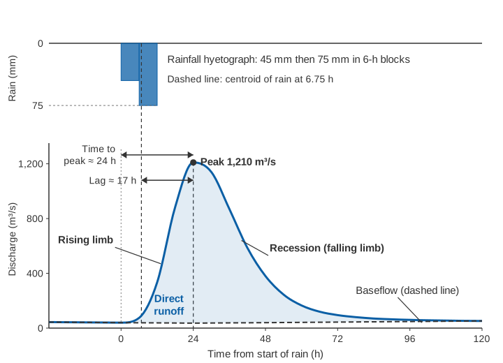
A flood hydrograph from a single storm has a recognisable shape. Before the storm the river carries a slowly declining flow. Rain falls, and after a delay the flow rises, reaches a maximum and then falls away, quickly at first and then more and more slowly, until it returns to a slowly declining flow again. Hydrologists name four parts:
- Rising limb. The part from the start of the rise to the peak. Its steepness is the rate at which discharge or level increases, in m³/s per hour or metres per hour.
- Peak. The highest discharge (or level) of the event, and the time at which it occurs. The peak and its timing are what most flood damage and most warning thresholds are about.
- Recession (falling limb). The part after the peak. It begins steep, while surface runoff is still draining, and then flattens. The US Department of Agriculture's National Engineering Handbook describes the point of inflection on the falling limb as the place where the recession curve begins [3].
- Baseflow. The flow sustained by groundwater, which would have been in the river even without the storm. The same handbook describes baseflow as water that infiltrates, reaches the water table, flows slowly and eventually reappears in the channel, and notes that it has little effect on flood peaks in small watersheds [3].
The water that makes up the flood itself, above the baseflow, is called direct runoff. It combines surface runoff and interflow (also called quick return flow): water that infiltrates but moves rapidly through the soil and returns to the surface. The WMO Guide to Hydrological Practices notes that interflow is often included as part of direct runoff, and that only in a simple two-component analysis, direct runoff plus baseflow, is it possible to separate an observed hydrograph into its parts [1].
Time terms: lag, time to peak and time of concentration
Three easily confused time measures describe how fast a catchment responds.
- Lag time. The WMO Guide defines basin lag (in the sense it uses) as the time from the centroid of rainfall to the peak of the hydrograph [1]. The National Engineering Handbook uses the same idea in hydrograph analysis: the interval between the centre of mass of the excess rainfall and the peak runoff rate [3]. Excess rainfall is the part of the rain that becomes direct runoff, after losses to interception, infiltration and depression storage.
- Time to peak. The time from the start of the rise (or the start of excess rainfall) to the peak. In the unit hydrograph method described in the WMO Guide it is the lag plus half the rainfall duration [1].
- Time of concentration (Tc). The time required for runoff to travel from the hydraulically most distant point in the catchment to the outlet [3]. For average natural catchments with roughly uniform runoff, the handbook relates it to the lag (L) by the approximation
L = 0.6 · Tc, both in hours [3]. How Tc is defined, estimated and used in design is the subject of time of concentration: why small catchments flood so fast.
One caution matters for anyone reading a single event. Lag is not a fixed property of a catchment. The handbook cites studies showing that lag varies from storm to storm with the amount, duration and intensity of rainfall, the growth stage of vegetation and the temporary storage available. For Deer Creek in Maryland (94.4 square miles, about 245 km²), measured lags for three storms were 5.06, 7.15 and 9.67 hours [3]. One event gives you one value; several events give you a range, and the range is the honest answer.
What the shape says about the catchment
Steep and narrow, or broad and flat
For the same volume of direct runoff, a short lag means the volume arrives in a short time, so the peak is high and the hydrograph is narrow. A long lag spreads the same volume over a longer time and gives a lower, broader peak. Snyder's synthetic unit hydrograph, described in the WMO Guide, expresses exactly this: the unit-hydrograph peak is proportional to catchment area divided by lag, Qp = C3 · A / tp, where C3 is an empirical constant [1]. The Guide also notes that unit hydrographs tend to become more peaked as runoff increases [1].
What makes lag short? In the empirical formulas in the WMO Guide, lag grows with stream and flow length and falls with average catchment slope [1]. The WMO flood forecasting manual singles out upland and urban catchments as the ones where response is fastest and lead time hardest to secure [2]. Small, steep hill catchments therefore tend to have short lags and sharp peaks, while large plains rivers have long lags and broad, slow hydrographs. Our article on flash floods and river floods looks at what this means for warning time.
Storage flattens and delays the peak
Anything that stores water temporarily, such as a reservoir, a lake, a wide floodplain or a wetland, lowers the peak and delays it. The 2018 Kerala floods provide a documented Indian example. In a peer-reviewed study of the Periyar basin (5,398 km², Kerala's longest river at 244 km), Sudheer and colleagues report a measured peak inflow to Idukki reservoir of 2,532 m³/s against a release of 1,614 m³/s on 15 August 2018 [4]. The reservoir clipped the peak passing through it. The study also shows the limits of that effect: much of the flood came from tributaries without reservoirs, driven by extreme rainfall on saturated soils. The observed peak at the downstream CWC gauging site was 8,800 m³/s [4]. The role of the reservoirs in that flood is examined in how dam spillways and gates work.
The simplest way to see the effect is a linear reservoir, one of the basic building blocks of conceptual hydrological models [1]: storage S is proportional to outflow O through a storage constant K (in hours), and the change in storage is inflow minus outflow. Move the slider to route the worked-example flood below through more and more storage. The peak falls and arrives later, and the outflow peak always sits on the falling limb of the inflow, at the moment the two curves cross, because that is when storage stops increasing.
Illustrative only: the inflow is the worked-example hydrograph from this article, not data from a real river or reservoir.
Antecedent conditions
The same storm on a dry catchment in June and a saturated one in August produces very different hydrographs. Wet soils let less water infiltrate, so more rain becomes direct runoff and the peak is higher. Standard methods build this in: the curve number method described in the WMO Guide uses a higher curve number, and so more runoff, under wet antecedent moisture conditions [1]. When you compare two floods, compare the rainfall and what fell in the preceding days.
Worked example: separating baseflow and measuring lag
The following is an illustrative example, built to show the method. It is not a record from a real station. Consider a catchment of 2,000 km² with a gauge at its outlet that reports discharge every six hours. A storm delivers 45 mm of rain between 0 and 6 h and 75 mm between 6 and 12 h, 120 mm in total. Before the storm the river carries about 40 m³/s and is slowly falling.
| Time (h) | Discharge (m³/s) | Baseflow line (m³/s) | Direct runoff (m³/s) |
|---|---|---|---|
| 0 | 40 | 40 | 0 |
| 6 | 75 | 39 | 36 |
| 12 | 335 | 38 | 297 |
| 18 | 885 | 37 | 848 |
| 24 | 1,210 | 36 | 1,174 |
| 30 | 1,140 | 37 | 1,103 |
| 36 | 870 | 38 | 832 |
| 42 | 585 | 39 | 546 |
| 48 | 380 | 40 | 340 |
| 54 | 245 | 41 | 204 |
| 60 | 165 | 42 | 123 |
| 66 | 120 | 43 | 77 |
| 72 | 95 | 44 | 51 |
| 78 | 80 | 45 | 35 |
| 84 | 70 | 46 | 24 |
| 90 | 64 | 47 | 17 |
| 96 | 60 | 48 | 12 |
| 102 | 57 | 49 | 8 |
| 108 | 55 | 50 | 5 |
| 114 | 53 | 51 | 2 |
| 120 | 52 | 52 | 0 |
Step 1: draw the baseflow line
The WMO Guide describes one of the simplest separation methods [1]. Extend the pre-storm baseflow trend forward to the time of the peak (point B). Then draw a straight line from B to the hydrograph at a point C, a fixed number of days N after the peak, where
N = (A / 2)^0.2 (N in days, A = drainage area in km²)For A = 2,000 km²:
N = (2000 / 2)^0.2 = 1000^0.2 = 3.98 ≈ 4 days = 96 hThe pre-storm flow was falling by about 1 m³/s every 6 hours, so extended to the peak at 24 h it reaches 36 m³/s (point B). Point C is 96 h after the peak, at 120 h, where the observed flow is 52 m³/s. The baseflow line therefore runs from 40 m³/s at 0 h down to 36 m³/s at 24 h, then up in a straight line to 52 m³/s at 120 h. It rises after the peak because the storm has recharged groundwater.
The Guide makes a point worth repeating: several separation methods are in common use, and using the same method consistently matters more than which method is chosen [1].
Step 2: volume and depth of direct runoff
Direct runoff is the observed discharge minus the baseflow line (last column). With equally spaced readings and zero direct runoff at both ends, the trapezoidal rule reduces to the sum of the ordinates times the time step:
Sum of direct runoff ordinates = 5,734 m³/s
Time step                      = 6 h = 21,600 s
Volume of direct runoff        = 5,734 × 21,600 = 123.9 million m³
Depth over catchment           = 123.9 × 10⁶ m³ / (2,000 × 10⁶ m²) = 0.062 m = 62 mm
Of 120 mm of rain, 62 mm left the catchment as direct runoff during the event: a runoff coefficient (direct runoff divided by rainfall) of 62 / 120 ≈ 0.52. The other 58 mm went to infiltration, storage and evaporation, part of it to return later as baseflow. Dividing every direct-runoff ordinate by 6.2 (the runoff depth in centimetres) would give the unit hydrograph for this storm, the same procedure the WMO Guide works through for its own example [1].
Step 3: lag time
The centroid of the rainfall is the rainfall-weighted mean time of the two blocks, taking each block at its midpoint:
Centroid = (45 mm × 3 h + 75 mm × 9 h) / 120 mm = (135 + 675) / 120 = 6.75 h
Lag      = time of peak − centroid = 24 − 6.75 = 17.25 h ≈ 17 h
Tc       ≈ L / 0.6 = 17.25 / 0.6 ≈ 29 h
Strictly, the centroid should come from the excess rainfall; if losses were concentrated early in the storm, the lag would be a little shorter. With six-hourly data the true peak lies somewhere between about 18 h and 30 h, so the lag is known only to within a few hours. For a catchment that responds in hours, the reporting interval must be much shorter than the lag, or the peak is simply missed.
Step 4: the recession
On the later part of the falling limb, flow decays roughly exponentially. The WMO Guide gives the standard form of a recession curve [1]:
Q(t) = Q0 · e^(−C (t − t0))Between 72 h (95 m³/s) and 96 h (60 m³/s):
C = ln(95 / 60) / 24 h = 0.460 / 24 = 0.019 per hour
Halving time = ln 2 / C = 0.693 / 0.019 ≈ 36 h
A small C means a slow, sustained recession. The recession rate, like the baseflow index (the ratio of baseflow to total flow), reflects catchment geology, and the WMO Guide describes studies that mapped recession indices against geological maps [1]. In forecasting, the Guide notes, recession analysis is used mainly for low flows [1].
The straight-line method suits event analysis by hand. For long continuous records, hydrologists more often use recursive digital filters. A widely used two-parameter filter is Eckhardt's:
b_k = [ (1 − BFImax) · a · b_(k−1) + (1 − a) · BFImax · y_k ] / (1 − a · BFImax), with b_k ≤ y_kwhere y is streamflow, b baseflow, a the recession constant and BFImax the maximum long-term ratio of baseflow to total flow that the filter can produce [5].
Why the rising limb matters most for warnings
Every part of the hydrograph is useful after the event. Only one part is useful during it. By the time the peak is visible on a chart, the water is already at its highest; the recession tells you about recovery, not danger. The rising limb is the window in which a warning can still be issued and acted on.
The WMO Manual on Flood Forecasting and Warning sets out the principle: lead time should be at least the minimum period needed for preparatory action. Householders may need one to two hours to move belongings or place sandbags; road diversions and moving livestock may need several hours; evacuation along large rivers may need days. In upland and urban catchments, the Manual says, the emphasis must be on real-time observation and rapid transmission of data [2].
Three practical points follow.
1. The rate of rise is itself a warning signal. In the illustrative example the flow rose by 43 m³/s per hour between 6 and 12 h, and by 92 m³/s per hour between 12 and 18 h. A rate-of-rise threshold can trigger an alert before any fixed level is reached. India's Central Water Commission reports a trend (rising, steady or falling) with each observed and forecast level in its daily flood bulletins, alongside each station's warning level, danger level and highest flood level [6].
2. Rising limbs accelerate, so straight-line extrapolation can be optimistic. The WMO Manual notes that where only water level records are available, extrapolation over a few hours is possible, depending on the catchment and the event [2]. But consider a village downstream in the example that floods above 600 m³/s. At 12 h the flow is 335 m³/s and has risen at 43 m³/s per hour over the previous six hours:
Extrapolated crossing = 12 h + (600 − 335) / 43.3 ≈ 12 + 6.1 = 18.1 h
Actual crossing (interpolated between 12 h and 18 h) = 12 + 6 × (600 − 335) / (885 − 335) ≈ 14.9 h
The simple extrapolation gave about three hours more than was actually available. Re-computing at every new reading, with short reporting intervals, narrows that gap.
3. Rainfall buys back the lag. From the threshold crossing at about 15 h to the peak at 24 h there were roughly nine hours. From the centroid of the rain to the peak there were about 17. The WMO Manual describes this progression: telemetered rain gauge or radar data add warning time beyond what river levels alone allow, and a rainfall forecast can add several hours more. In its example from upland catchments in the south of France, a catchment response of about 10 hours plus a 6 to 12 hour rainfall forecast gives 15 to 20 hours of lead time [2]. Our explainer on how a flood early warning system works describes how these pieces fit together.
Common mistakes when reading hydrographs
- Treating one event as typical. Lag and peakedness change with storm size, rainfall pattern and soil moisture [1][3]. Analyse several events.
- Reading a discharge hydrograph as if it were measured. Most discharge records are water levels converted through a rating curve, and floods are where that conversion is least certain, including the loop between rising and falling limbs. See rating curves and their uncertainty.
- Sampling too coarsely. A six-hourly or daily record cannot resolve a catchment that responds within a few hours.
Key points
- A flood hydrograph has a rising limb, a peak, a recession and an underlying baseflow; direct runoff is the flow above the baseflow.
- Lag time (rainfall centroid to peak) and peak shape describe how fast a catchment responds; a short lag gives a high, narrow peak for the same runoff volume.
- Lag is not constant: it varies from storm to storm, so use several events.
- Straight-line baseflow separation, with N = (A/2)^0.2 days, gives the runoff volume and the runoff coefficient of an event; use one method consistently.
- The rising limb is the only part of the flood in which warnings can still help. Its rate of rise, short reporting intervals and upstream rainfall data are what extend the warning time.
Turning past hydrographs into useful warning thresholds needs continuous, high-frequency records of water level and velocity from the river itself, together with rainfall upstream. That is the focus of our river monitoring work, and of PRAVAAH, an automatic water level recorder (AWLR) and surface velocity radar (SVR) that measures water level and surface velocity continuously, so that the rising limb of each event is recorded as it happens. For the particular challenges of steep catchments, see river monitoring in hill and Himalayan catchments.
References
- World Meteorological Organization, Guide to Hydrological Practices, Volume II: Management of Water Resources and Application of Hydrological Practices, WMO-No. 168, sixth edition, WMO, 2009 (Chapter 6, hydrograph analysis and unit hydrographs; Chapter 7, flow recession). WMO PDF.
- World Meteorological Organization, Manual on Flood Forecasting and Warning, WMO-No. 1072, WMO, 2011 (Section 2.1.4, forecast lead time). WMO PDF.
- United States Department of Agriculture, Natural Resources Conservation Service, National Engineering Handbook, Part 630 Hydrology, Chapter 15: Time of Concentration, 210-VI-NEH, USDA NRCS, 2010. directives.nrcs.usda.gov (PDF).
- K. P. Sudheer, S. Murty Bhallamudi, B. Narasimhan, J. Thomas, V. M. Bindhu, V. Vema, C. Kurian, Role of dams on the floods of August 2018 in Periyar River Basin, Kerala, Current Science 116(5), 780–794, 2019. doi:10.18520/cs/v116/i5/780-794.
- K. Eckhardt, Technical note: How physically based is hydrograph separation by recursive digital filtering?, Hydrology and Earth System Sciences 27, 495–499, 2023. doi:10.5194/hess-27-495-2023.
- Central Water Commission, Flood Forecast Monitoring Directorate, Flood Situation Summary, daily bulletin (example: Bulletin No. 31, 31 May 2020), Government of India, 2020. cwc.gov.in.