
Why Indian reservoirs lose storage: sediment and siltation explained
How rivers carry sediment into a reservoir, where it settles, how much storage Indian reservoirs lose each year, and how and how often the capacity curve should be checked.

Every reservoir starts losing storage on the day it begins to fill. The river keeps delivering sand, silt and clay, the still water behind the dam lets most of it settle, and each cubic metre of sediment replaces a cubic metre of water. The loss is slow and out of sight, so the elevation–area–capacity table in the control room can stay the same for decades while the reservoir changes. This article explains where the sediment comes from, where it settles, how fast Indian reservoirs are losing capacity, what that does to dead storage, rule curves and the flood cushion, and how the capacity curve is measured again.
How a river carries sediment
Sediment moves in two broad ways. The WMO Guide to Hydrological Practices describes grains that are "swept away" from the bed and kept in suspension, and grains that slide, roll or hop (saltate) along or near the bed. For convenience it divides sediment discharge into suspended-sediment discharge and bed-material discharge, while noting that the two happen together and there is no sharp line between them [1].
- Suspended load is the fine sand, silt and clay carried within the flow. It is what makes a monsoon river brown, and it is what gauging stations normally sample, by taking water samples and measuring concentration.
- Bed load is the coarser sand, gravel and boulders moving along the bed. It is hard to measure. The Indian standard on sedimentation in reservoir planning, IS 12182:1987, notes that where bed load is not measured it is often estimated as 5 to 20 percent of the suspended load, and asks for measurement where high bed loads are expected [2].
Because sediment load varies with discharge, sediment yield is estimated from a sediment rating curve (concentration or load against discharge) combined with a flow-duration curve, as both IS 12182 and IS 5477 (Part 2) describe, or from the sediment already measured in existing reservoirs [2][3].
Where the sediment settles
When the river enters the reservoir, its cross-section widens and the velocity falls, and the sediment begins to drop out in order of size. The CWC Compendium on Sedimentation of Reservoirs in India (2020) describes the main patterns [4]:
- Delta at the head. The coarsest fraction settles quickly where the river meets the reservoir and builds a delta. Over time the delta grows and advances towards the dam.
- Fine sediment towards the dam. Silt and clay travel further. Turbid inflow is denser than the clear water in the reservoir, so it can sink and run along the bottom as a density current (a "stratified flow"), carrying fines to the deepest part near the dam. This produces a wedge of deposits that is thickest at the dam.
- Tapering and uniform deposits occur in other reservoirs depending on shape, operation and the sediment supplied.
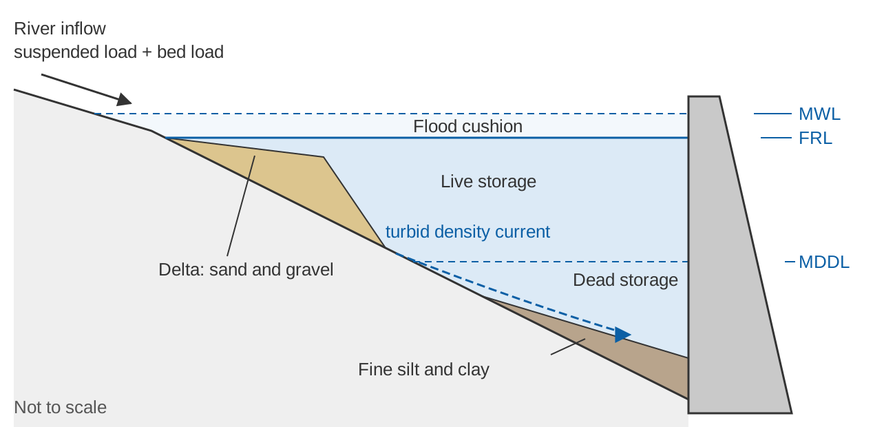
The last point of the caption is the most important lesson of Indian resurveys. Projects planned up to the mid-1960s commonly assumed that sediment would first fill the dead storage (the volume below the lowest outlet or minimum drawdown level, set aside for sediment) before touching the live storage (the usable volume between MDDL and FRL). Surveys showed this to be wrong: deposition occurs throughout the depth of the reservoir and reduces capacity at every elevation [4]. IS 12182 records the same conclusion: silt occupies live storage as well as dead storage [2].
Trap efficiency: how much stays behind
Not all the inflowing sediment stays. Trap efficiency is the ratio of sediment deposited to sediment that flowed in over a period [2]. Gunnar Brune analysed 44 reservoir records and found that the ratio of reservoir capacity to mean annual inflow (C/I) predicts trap efficiency much better than the ratio of capacity to catchment area. He published a median curve with upper and lower envelopes. Desilting basins could trap more than 90 percent even at very low C/I, while reservoirs that are often dry trapped roughly 10 to 40 percent [5]. IS 12182 adopts Brune's curve and Churchill's curve for computing trap efficiency [2].
A commonly used fit to Brune's median curve, attributed to Heinemann (1981) and quoted by Lewis et al. [6], is given below. It reproduces the worked example in IS 12182, where a capacity–inflow ratio of 0.04 is read from the median curve as 75 percent trap efficiency [2]; the equation gives 76 percent.
TE (%) = 100 × (C/I) / (0.012 + 1.02 × C/I)

C = reservoir capacity (m³)
I = mean annual inflow volume (m³ per year)
C/I = 0.01  →  TE ≈ 45 %
C/I = 0.1   →  TE ≈ 88 %
C/I = 1.0   →  TE ≈ 97 %
Two cautions follow. First, as a reservoir fills with sediment, C falls and so does trap efficiency, which is why IS 12182 notes that "life" calculations commonly ignored the change in trap efficiency towards the end of the period [2]. Second, the curve was built from reservoirs in the United States. A study of the Burdekin Falls Dam in tropical Australia, which receives highly variable summer-dominant inflows, measured trap efficiencies of 50 to 85 percent, considerably less than the Brune and Churchill curves predicted, because floods pass through quickly [6]. Monsoon-fed Indian reservoirs also receive most of their inflow in one season, so a curve value is a starting estimate, not a measurement.
How fast Indian reservoirs are losing storage
The CWC compendium (2020) compiled capacity survey results for 369 reservoirs. From hydrographic surveys of 264 reservoirs, it computed an average annual loss of 0.95 percent of gross storage. From the reservoirs with usable data for each zone, the average annual loss was 2.39 percent of dead storage (141 reservoirs) and 0.67 percent of live storage (126 reservoirs). Satellite remote sensing surveys of 86 reservoirs gave an average annual loss of 0.73 percent of live storage [4]. These are averages weighted by size (total annual loss divided by total storage), and the range is wide: the annual loss of gross storage ran from 0.03 to 21.03 percent [4].
For comparison, IS 12182 classes a new reservoir's sedimentation problem as insignificant if the expected annual deposit is less than 0.1 percent of gross capacity, serious if it is more than 0.5 percent, and significant in between [2]. By that yardstick, 117 of the 264 surveyed reservoirs (65 + 52) are losing storage at a rate the standard would call serious. Worldwide, ICOLD Bulletin 147 found a mean reservoir sedimentation rate of 0.8 percent of original storage capacity per year [7], and the CWC compendium cites estimates of 0.5 to 1.0 percent a year [4].
The compendium also expresses sedimentation as the depth of sediment per unit catchment area per year. Its median values from hydrographic surveys (1 mm per year equals 1,000 m³ per km² per year) were [4]:
| Region (CWC classification) | Median rate (mm/yr) |
|---|---|
| West flowing rivers beyond Tapi and south Indian rivers | 2.07 |
| West flowing rivers up to Narmada | 0.86 |
| Indus and Ganga plains | 0.72 |
| East flowing rivers up to Godavari | 0.68 |
| Narmada and Tapi basins | 0.651 |
| Deccan peninsular region | 0.44 |
| Himalayan region (Indus, Ganga and Brahmaputra basins) | 0.42 |
The compendium uses medians because a few extreme reservoirs pull the averages up. It also reports that the observed rate exceeded the design rate in most of the 105 reservoirs for which both were known, that sedimentation tends to be fastest in the first years of operation and then slows, and that some reservoirs past their planned life still provide substantial benefits [4]. Individual Himalayan reservoirs can still lose storage quickly, so these regional medians are no substitute for a survey of the reservoir itself.
What lost storage means for operation
The elevation–area–capacity curve
Every reservoir is operated through its elevation–area–capacity curve, a table that gives the water-spread area and the stored volume at each level. Sediment lowers the volume at every level, and once the bottom fills, the level at which the stored volume becomes zero (the new zero elevation) rises. A curve that has not been updated overstates the water held at any given level.
Dead storage
IS 5477 (Part 2) describes dead storage as the volume equivalent to the sediment expected to deposit during the design life of the structure [3]. The CWC compendium notes that the older practice was to size it for 100 years of sediment at a design rate [4]. IS 12182 defines the feasible service time (the period during which the reservoir still gives part of its planned benefit) as customarily ending when the new zero elevation reaches the sill of the outlet that serves the purpose, and sets design minimums: for irrigation projects a full service time of at least 50 years and a feasible service time of at least 100 years; for hydropower supplying a grid, 25 and 70 years [2]. Because the dead storage fills from the bottom, outlet and intake sills are the places where sediment first becomes an operational problem.
Rule curves and the flood cushion
A rule curve is the target level planned for a reservoir at different times of the year under given probabilities of inflow and demand. IS 7323:1994 describes rule curves for the filling and depletion periods, and the permanent allocation of flood space at the top of the conservation pool where floods can occur at any time of year [8]. Both are defined as levels, but both are designed as volumes. When sediment reduces the volume between two levels, the same rule curve stores less water for irrigation, drinking water and power, and the same flood space absorbs less of an incoming flood.
Operators also estimate inflow as outflow plus the change in storage, read from the change in level through the capacity curve, so a stale curve biases that calculation in every flood. This is one reason accurate level records and an up-to-date curve go together; see what dam operators need to measure and why.
How capacity is resurveyed
Hydrographic (bathymetric) survey
A boat with an echo sounder measures depth along planned lines across the reservoir, while a differential GPS (DGPS) fixes its position against a base station set on a known benchmark. Software links the depth and position records to give X, Y and Z points on a grid, from which the bed surface, and then the capacity at each level, are computed [4]. Older surveys used theodolites, plane tables, sextants and sounding rods; the compendium notes that a conventional survey of a major reservoir such as Hirakud could take up to three years, and that DGPS-based bathymetry saves time and gives more reliable results [4]. A bathymetric survey is the only method that measures the whole reservoir, including the dead storage zone.
Remote sensing: the water-spread method
As a reservoir draws down after the monsoon, its shoreline shrinks. A satellite image on a date with a known reservoir level gives the water-spread area at that level, and a series of images through the drawdown season gives area at many levels. A study of Gobind Sagar (Bhakra) in Himachal Pradesh, for example, used the Normalized Difference Water Index on Landsat 8 images to separate water from land, took the matching reservoir levels from India-WRIS, and computed the volume between successive levels with the prismoidal ("modified trapezoidal") formula [9]:
NDWI = (Green − NIR) / (Green + NIR)

V = (h / 3) × (A1 + A2 + √(A1 × A2))

h      = height between two successive levels (m)
A1, A2 = water-spread areas at those levels

Example: A1 = 20 km², A2 = 24 km², h = 2 m
V = (2 / 3) × (20 + 24 + √480) = (2 / 3) × 65.9 = 43.9 km²·m = 43.9 million m³
Comparing the revised capacities with the original curve, that study estimated a loss of 783.38 million m³ (10.71 percent) of capacity between 467.38 m and 511.32 m since first impoundment in 1963, an average of 14.24 million m³ a year [9]. The method is fast and cheap, but it only sees levels that the reservoir actually reaches on cloud-free image dates, so it cannot measure capacity below the lowest observed level, which is usually around MDDL [4][9].
How often to recheck the curve
The CWC compendium states that the normal frequency of capacity surveys is supposed to be about five years. It also records the recommendation of the national working group on satellite-based sedimentation assessment: a composite survey (hydrographic below MDDL, satellite above) every 10 years, a mid-term satellite survey every 5 years, and every 3 years for reservoirs that silt quickly [4].
IS 12182 adds a useful caution: conclusions about sedimentation rate should be drawn from two surveys only when they differ by at least about 10 percent of capacity, otherwise survey error can distort the result [2]. Together these suggest a practical approach: update the operating curve as often as the survey methods allow, but judge the long-term rate from surveys far enough apart for the change to stand out above the measurement error.
Worked example: annual loss and useful life
Illustrative numbers, chosen to sit within the ranges quoted above.
A reservoir has a gross capacity of 500 million m³ (MCM) at FRL, of which 58.9 MCM lies below MDDL (dead storage) and 441.1 MCM is live. Mean annual inflow is 1,200 MCM. Gauging upstream gives a suspended load of 2.4 million tonnes a year.
1. Total sediment inflow
   Bed load (assume 15 % of suspended, within the 5–20 % of IS 12182)
   = 0.15 × 2.4 = 0.36 Mt/yr
   Total = 2.4 + 0.36 = 2.76 Mt/yr

2. Trap efficiency (Brune median curve)
   C/I = 500 / 1,200 = 0.417
   TE = 100 × 0.417 / (0.012 + 1.02 × 0.417) = 95.3 %
   Trapped = 2.76 × 0.953 = 2.63 Mt/yr

3. Volume of deposits (assume dry density 1.2 t/m³)
   V = 2.63 / 1.2 = 2.19 MCM/yr

4. Annual loss of gross storage
   2.19 / 500 × 100 = 0.44 % per year   (IS 12182: "significant")

5. Time to lose half the gross capacity
   250 / 2.19 = 114 years at a constant rate
   (recomputing TE each year as C falls: 116 years)
Now the distribution. Under the old assumption that all sediment goes into dead storage, the dead storage would be full in 58.9 / 2.19 = 27 years. Suppose instead, consistent with the surveys, that 60 percent settles below MDDL and 40 percent within the live zone:
Below MDDL:   0.6 × 2.19 = 1.32 MCM/yr   → dead storage full in 58.9 / 1.32 ≈ 45 years
In live zone: 0.4 × 2.19 = 0.88 MCM/yr   → 0.88 / 441.1 = 0.20 % of live storage per year
After 30 years: 65.8 MCM deposited; dead storage 19.4 MCM left (67 % lost);
                live storage 414.8 MCM (6.0 % lost); gross 434.2 MCM (13.2 % lost)
The live zone loses storage from the first year, and the dead storage is used up well within the century that older designs assumed. If the annual gross loss were the CWC national average of 0.95 percent of original capacity instead of 0.44 percent, half the gross capacity would be gone in 50 / 0.95 ≈ 53 years. The calculator below lets you try other values.
What can be done
The compendium lists measures before construction (site selection, staged dam height, outlets at several levels) and after it (passing sediment-laden floods through outlets, sluicing or dredging, and catchment soil conservation), with their limits: sluices scour only a narrow channel, dredging suits mainly small reservoirs, and catchment treatment is slow to show results [4]. Each depends on knowing how much sediment arrives and where it settles.
Key points
- Rivers carry sediment as suspended load (fine sand, silt and clay in the flow) and bed load (coarser material along the bed). Unmeasured bed load is often taken as 5 to 20 % of the suspended load.
- In a reservoir, coarse sediment builds a delta at the head and fines travel towards the dam, partly as density currents. Deposits form at every depth, so live storage is lost as well as dead storage.
- Brune's curve links trap efficiency to the capacity–inflow ratio, but it can overestimate trapping where inflows are highly seasonal.
- The CWC compendium (2020) reports average annual losses of 0.95 % of gross, 2.39 % of dead and 0.67 % of live storage from hydrographic surveys, and 0.73 % of live storage from satellite surveys.
- Lost storage shifts the elevation–area–capacity curve, raises the zero elevation towards outlet sills, and reduces the water held under every rule-curve level and flood-space allocation.
- Resurveys combine bathymetry (the whole reservoir) with the satellite water-spread method (the live zone); CWC guidance points to a composite survey every 10 years with satellite surveys every 5 years, or every 3 years for fast-silting reservoirs.
At ClimMaTech we work on the measurement side of this problem: the reservoir levels, inflows and rainfall records that capacity curves, rule curves and sediment budgets depend on. To see how we approach monitoring at dams and reservoirs, visit our dam and reservoir solutions page.
References
- World Meteorological Organization, Guide to Hydrological Practices, Volume I: Hydrology – From Measurement to Hydrological Information, WMO-No. 168, 2008 edition, updated in 2020, section 5.5 (sediment discharge and yield). WMO Hydrology Publications page; full text: copy hosted by Agência Nacional de Águas, Brazil.
- Bureau of Indian Standards, IS 12182:1987 Guidelines for determination of effects of sedimentation in planning and performance of reservoirs, BIS, 1987. archive.org (archived copy).
- Bureau of Indian Standards, IS 5477 (Part 2):1994 Methods for fixing the capacities of reservoirs, Part 2: Dead storage, BIS, 1994. archive.org (archived copy).
- Central Water Commission, Compendium on Sedimentation of Reservoirs in India, Watershed and Reservoir Sedimentation Directorate, CWC, Ministry of Jal Shakti, 2020. cwc.gov.in.
- G. M. Brune, Trap efficiency of reservoirs, Eos, Transactions American Geophysical Union 34(3), 407–418, 1953. doi:10.1029/TR034i003p00407. USGS record.
- S. E. Lewis, Z. T. Bainbridge, P. M. Kuhnert, B. S. Sherman, B. Henderson, C. Dougall, M. Cooper, J. E. Brodie, Calculating sediment trapping efficiencies for reservoirs in tropical settings: A case study from the Burdekin Falls Dam, NE Australia, Water Resources Research 49, 1017–1029, 2013. doi:10.1002/wrcr.20117.
- International Commission on Large Dams, Sedimentation and Sustainable Use of Reservoirs and River Systems, ICOLD Bulletin 147, CRC Press, 2024 (preprint 2009). Publisher page.
- Bureau of Indian Standards, IS 7323:1994 Operation of reservoirs – Guidelines, BIS, 1994. archive.org (archived copy).
- S. Singh, M. K. Dhasmana, V. Shrivastava, V. Sharma, N. Pokhriyal, P. K. Thakur, S. P. Aggarwal, B. R. Nikam, V. Garg, A. Chouksey, P. R. Dhote, Estimation of revised capacity in Gobind Sagar reservoir using Google Earth Engine and GIS, International Archives of the Photogrammetry, Remote Sensing and Spatial Information Sciences XLII-5, 589–595, 2018. doi:10.5194/isprs-archives-XLII-5-589-2018.