
Catchment area vs watershed: delineating a basin from a DEM
What catchment, watershed, river basin and command area mean, how a basin is traced from a digital elevation model step by step, and where the method goes wrong in Indian terrain.

Before a river gauge can tell you anything beyond the water level, someone has to answer a plain question: how much land drains to this point? That number is the catchment area, and it goes into most calculations that follow. Reports use catchment area vs watershed, river basin and drainage basin almost interchangeably, and the number is increasingly computed from a digital elevation model (DEM) rather than traced on toposheets. This article sorts out the terms, walks through watershed delineation from a DEM with a worked example, and shows where the method goes wrong in the Himalaya and on the Indo-Gangetic plains.
Catchment area vs watershed: is there a difference?
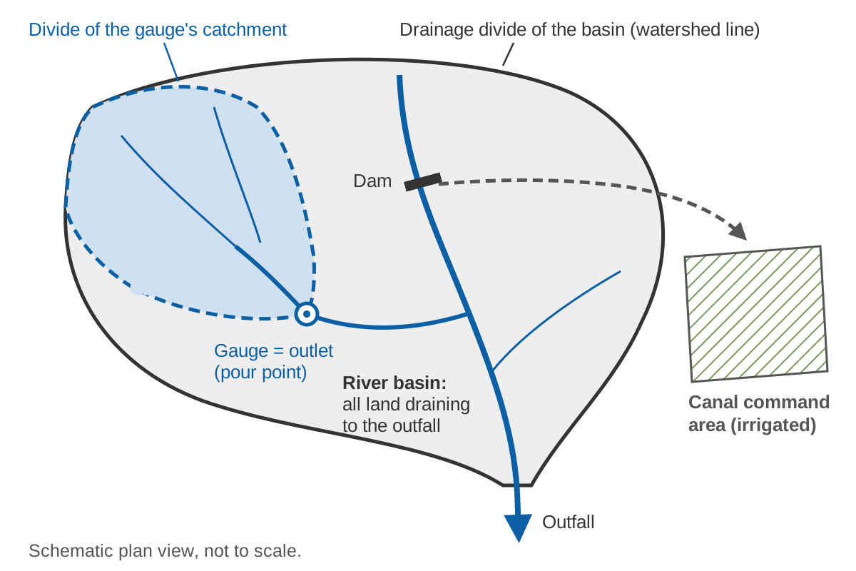
For most purposes, no. The International Glossary of Hydrology published by WMO and UNESCO lists "basin" with the synonyms drainage basin, catchment, river basin and watershed, marking "watershed" in this sense as United States usage, and defines it as an "area having a common outlet for its surface runoff" [1]. The line that separates adjacent basins is the watershed divide, also called the drainage divide or water parting [1]. Catchment area is the size of that area, in km² or hectares [1].
In India, "watershed" also names a size class. The India-WRIS hierarchy runs water resources region, basin, sub-basin, watershed, sub-watershed and micro-watershed, with 6 regions, 25 basins and 101 sub-basins [2]. When a document says "watershed", check which sense it means.
| Term | Meaning | Note |
|---|---|---|
| Catchment, drainage basin, basin | Area whose surface runoff leaves through one outlet [1] | Can be defined for any point on a river |
| Catchment area, drainage area | The size of that area | The number used in calculations |
| Watershed | Same as catchment in US usage [1]; in India-WRIS also a unit below the sub-basin [2] | Check the sense |
| Drainage divide, watershed divide | Boundary line between adjacent basins [1] | Crosses the drainage only at the outlet [2] |
| River basin | Catchment of a whole river at its outfall | 25 basins under India-WRIS [2] |
| Command area | Land served by an irrigation system [4][5] | Not a hydrological unit |
Catchment area vs river basin
A river basin is the catchment of an entire river at its outfall into the sea, a lake or a larger river. A catchment can be defined at any point: a gauge, a dam, a bridge. WMO's Guide to Hydrological Practices defines the basin as "the area that receives precipitation and, after hydrological processes resulting in losses and delays, leads it to an outflow point" [3]. The River Basin Atlas of India notes that the size of a hydrological unit is set by the point of interception, such as a dam, barrage, weir or observation site, from thousands of km² for a multipurpose project to a few hectares for a farm pond [2].
Basin counts depend on who drew them: 20 basins in the first delineation of 1949, made from Survey of India toposheets, then 35, 24 and 34 in later schemes, and 25 under India-WRIS, drawn from a DEM [2]. Quote a basin area with its classification.
Catchment vs command area
Command area is an irrigation term, not a hydrological one. The Central Water Commission defines the culturable command area (CCA) as "the geographical area which can be irrigated from an irrigation system and is fit for cultivation", and classifies schemes as major (CCA above 10,000 ha), medium (2,000–10,000 ha) and minor (up to 2,000 ha) [4]. The gross command area is the total area that can be commanded from a project without considering the water available, and the CCA is the gross command area less the non-culturable land [5].
The catchment above a dam supplies the water; the command area uses it, and because canals can cross a divide, it may lie in another basin. Never use a command area in a runoff calculation.
How watershed delineation from a DEM works
A DEM is a grid of elevation values with regular spacing [3]. The standard sequence was set out by Jenson and Domingue at the USGS EROS Data Center: a conditioning phase produces a DEM with depressions filled, a flow direction for every cell and a flow accumulation for every cell, from which drainage lines and the watershed of any chosen point follow [6].
1. Prepare the DEM
Clip the DEM with a margin beyond the expected divide and project it to a metric coordinate system. The Shuttle Radar Topography Mission (SRTM), flown in February 2000, produced elevation data at 1 arc-second, about 30 m [10][19]. Its original release had voids where radar shadow prevented reliable heights, notably in mountains such as the Himalaya [10]. Gaps inside the area of interest must be filled before routing flow [13].
2. Remove the sinks: fill or breach
A sink is a cell, or group of cells, entirely surrounded by higher cells. Most are artefacts of how the DEM was made, but some are real, and spurious sinks interrupt continuous flow across the surface [10]. Filling raises the cells in a sink until an outflow point is reached [10]; breaching carves a channel through the blocking cells; hybrid methods combine the two [11][12]. A least-cost search, used in GRASS GIS r.watershed, routes flow out of depressions without altering the DEM, so it needs no filling [11][13].
The choice matters. On radar DEMs of central Panama, streams from the least-cost method lay closer to GPS points on real rivers than streams from sink filling, which along one river section had changed 92 % of the elevation values [11]. And many depressions are real wetlands that careless filling erases [15].
3. Flow direction (D8)
The D8 method sends all flow from each cell to one of its eight neighbours, in the direction of steepest downward slope. It was introduced by O'Callaghan and Mark and has been widely used ever since [7][8]. Slope is the drop divided by the distance between cell centres, which for a diagonal neighbour is √2 times the cell size. HydroSHEDS, the global hydrography derived from SRTM [9], stores directions with the codes E = 1, SE = 2, S = 4, SW = 8, W = 16, NW = 32, N = 64 and NE = 128 [10]; GRASS r.watershed numbers them 1 to 8 counter-clockwise from north-east [13]. Check the convention before mixing tools.
Cells on a flat, including filled sinks, have no downhill neighbour. They are made to drain towards a neighbour of equal elevation that already has a direction [8]. D8 cannot split flow between two cells, so it introduces grid bias on hillslopes and cannot represent braided rivers [8][10]. D-infinity and multiple-flow-direction methods address this [8][13]. The methods differ most on hillslopes, where contributing areas are small, and give similar results for large contributing areas [8].
4. Flow accumulation
Flow accumulation is the number of cells that drain through each cell. Multiplied by the cell area, it gives the upslope or contributing area [8][10].
5. Stream threshold
Cells whose accumulation exceeds a threshold, sometimes called the critical support area, are treated as channels [8]. In r.watershed the threshold is the minimum size of an exterior basin in cells, and very low values greatly increase run time [13]. There is no universal value: compare the extracted network with mapped streams or imagery and adjust.
6. Snap the pour point
The pour point (outlet) is the cell whose catchment you want. A GPS fix taken on the bank often falls in a hillslope cell beside the channel, and the GRASS manual warns that an outlet on a hillslope yields only a thin sliver of land [14]. Snapping tools move the point to the nearest stream cell [17] or to the highest-accumulation cell within a search distance. Too large a distance can jump to a neighbouring stream, so always check the result.
7. Delineate and calculate
Trace every cell that drains to the outlet, convert the result to a polygon and compute its area.
A worked D8 example
The figure below uses a 6 × 5 grid of 30 m cells. All numbers are illustrative.
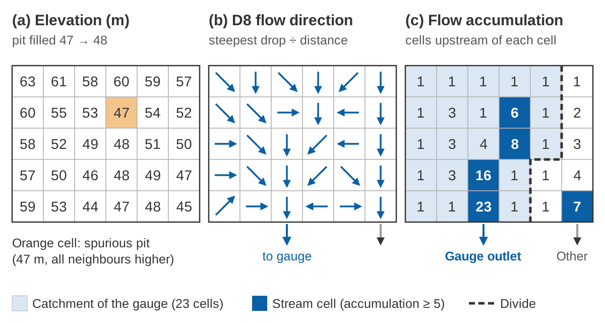
Filling the pit. The cell in row 2, column 4 is 47 m, and all eight neighbours are higher. Its lowest neighbour is 48 m (row 3, column 4), so filling raises it to 48 m. It now drains to that neighbour, which in turn drains south-west to the 46 m cell, a slope of (48 − 46) ÷ 42.4 = 0.047.
Choosing a direction. Take the 49 m cell in row 3, column 3. The diagonal distance is 30 × √2 = 42.4 m. The neighbours lower than it are:
East        48 m   (49 − 48) / 30.0 = 0.033
South-east  48 m   (49 − 48) / 42.4 = 0.024
South       46 m   (49 − 46) / 30.0 = 0.100   <- steepest
North-east  48 m   (49 − 48) / 42.4 = 0.024   (the filled pit)
The steepest drop is to the south, so the cell gets code 4.
Accumulating and delineating. Counting every cell that drains through each cell (itself included) gives panel (c). With a threshold of 5, the stream cells are those with 6, 8, 16 and 23 upstream cells, plus the 7-cell stream on the right. The outlet cell at the bottom has 23 cells upstream:
Catchment area = N × (cell size)²
               = 23 × (30 m)² = 23 × 900 m² = 20,700 m² = 2.07 ha
Try it below. Tap the cell to the right of the outlet (where a GPS fix on the bank might fall) with snapping off, and the catchment shrinks to one cell. Tap a cell near the divide with snapping on, and the outlet can jump to the wrong stream.
The grid and areas are illustrative, for learning the method only.
How to calculate catchment area
Count the cells that drain to the outlet and multiply by the area of one cell: N × Δx² on a projected grid of square cells. On a geographic grid (cells in arc-seconds), cell area shrinks with latitude, which is why HydroSHEDS supplies a separate accumulation grid in true area [10].
The size of the error is easy to show. A degree of latitude is 111.111 km [3], so:
1 arc-second north–south = 111,111 m ÷ 3,600 = 30.86 m
1 arc-second east–west at 31° N = 30.86 m × cos 31° = 30.86 × 0.857 = 26.46 m
True cell area at 31° N = 30.86 × 26.46 = 816 m²
Assuming 30 m × 30 m = 900 m² overstates the area by 900 ÷ 816 = 1.10, i.e. about 10 %
Compute areas in an equal-area projection, or with per-cell areas, and compare the result with any published figure for the site, such as the basin catchment areas tabulated in the River Basin Atlas [2].
How to do watershed delineation in QGIS
Use the GRASS tools in the Processing Toolbox: r.watershed builds the drainage and stream maps, and r.water.outlet cuts out the catchment of your gauge. The standalone QGIS installer for Windows installs GRASS, and Processing uses that copy [16]. The steps:
- Load the DEM and reproject it to a metric coordinate system suitable for your area.
- Fill no-data gaps (r.fillnulls) [13].
- Run r.watershed with a threshold to get flow accumulation, drainage direction and streams. Sink filling is not needed, because the module uses a least-cost search; the -s option gives single (D8) flow direction instead of the default multiple flow direction [13].
- Find your gauge on the streams map and note the coordinates of the stream cell, not the bank.
- Run r.water.outlet with the drainage direction map and those coordinates; cells with value 1 form the catchment [14].
- Convert the catchment raster to a polygon and calculate its area in an equal-area or suitable projected system.
Other free tools follow the same logic. WhiteboxTools includes a "Jenson" snap that moves outlets to the nearest stream cell [17]; TauDEM provides pit removal, contributing area, a channel threshold based on stream drops, and watershed delineation [18]. Results differ between tools with how each handles sinks [11].
Pitfalls in Himalayan terrain
- Voids and narrow gorges. SRTM voids from radar shadow affected the Himalaya [10]. A gorge narrower than about 90 m can appear closed on a 90 m surface, and HydroSHEDS had to carve through such barriers [10]. Sink filling in mountains can also shift confluences [11].
- Glaciers. SRTM shows the ice surface of February 2000 [19]. Glaciers worldwide lost 267 ± 16 gigatonnes per year over 2000–2019, and thinning rates of glaciers outside the ice-sheet peripheries doubled over those two decades [20]. Check divides across ice fields against recent imagery. How melt shapes river flow is covered in snow and glacier melt.
- Transboundary catchments. Large parts of these catchments lie outside India, and the Atlas tabulates the Indus basin only up to the border [2]. A DEM clipped at the border gives the wrong area for any gauge downstream.
| Basin | Total area (km²) | Area in India (km²) | Share in India |
|---|---|---|---|
| Indus | 1,165,500 | 321,289 | 321,289 ÷ 1,165,500 = 28 % |
| Ganga | 1,086,000 | 861,452 | 861,452 ÷ 1,086,000 = 79 % |
| Brahmaputra | 580,000 | 194,413 | 194,413 ÷ 580,000 = 34 % |
Areas from the River Basin Atlas of India [2]; shares calculated here.
For hill sites more generally, see river monitoring in hill and Himalayan catchments.
Pitfalls in flat Indo-Gangetic terrain
- No clear divide. The boundary may be hard to find where a stream rises in a very flat-bottomed valley or marshland [3], and small units are hard to delineate in plains with incipient drainage [2].
- Vegetation and resolution. Radar DEMs partly measure the vegetation top, so vegetated floodplains are prone to errors [10]. In the Panama study, drainage paths from 90 m SRTM lay about 100 m from reference points, against 34.4 m for a 10 m radar DEM [11].
- Roads, embankments and bridges. Clearings for roads can create false depressions that look like valleys, while bridges and dense housing can form false barriers [10]. Embankments and dams block flow paths in the DEM, and sink filling behind them lifts and flattens the land upstream; in coastal plains it can produce long straight artificial streams [10][11].
- Braided rivers and canals. D8 allows one direction per cell, so braided channels cannot be resolved, and canal diversions needed manual correction even in HydroSHEDS [10]. India-WRIS combined the DEM with drainage, water-body, rail and road data and validated boundaries against contours [2]. Stream burning, lowering the DEM along mapped rivers, is a common fix where a reliable river map exists [10].
How a gauge site's catchment area is used
Runoff depth and specific discharge. Discharge per unit area of a basin is specific discharge [1], which lets you compare rivers of different sizes. For an illustrative gauge with a mean flow of 40 m³/s and a catchment of 850 km²:
Specific discharge = 40 m³/s ÷ 850 km² = 0.047 m³/s per km² = 47 L/s per km²
Annual runoff depth = 40 × 365 × 86,400 m³ ÷ (850 × 10⁶ m²) = 1.48 m = 1,484 mm
Peak flow estimates. The rational method expresses peak storm runoff as the product of catchment area, peak rainfall rate and a runoff coefficient [1]; the rainfall rate is taken for a storm lasting the catchment's time of concentration. With intensity in mm/h and area in km², 1 mm/h over 1 km² is 0.001 m × 10⁶ m² ÷ 3,600 s = 0.278 m³/s, hence:
Q = C × i × A ÷ 3.6
Illustrative: C = 0.5, i = 40 mm/h, A = 12 km² → Q = 0.5 × 40 × 12 ÷ 3.6 = 66.7 m³/s
Transferring flows. The drainage-area ratio method equates the ratio of streamflows at two sites to the ratio of their drainage areas, usually with an exponent of one; a USGS analysis of Texas streams found exponents of about 0.89 down to 0.70 depending on the flow percentile [21]. For an illustrative site of 620 km² upstream of the 850 km² gauge above:
Ratio = 620 ÷ 850 = 0.729
Exponent 1.00:  40 × 0.729        = 29.2 m³/s
Exponent 0.89:  40 × 0.729^0.89   = 30.2 m³/s
Exponent 0.70:  40 × 0.729^0.70   = 32.1 m³/s
The method assumes similar runoff per km² at both sites, which fails where rainfall and snowmelt change sharply over short distances.
Models. In our study of ten catchments grouped by physical and climatic attributes, with model parameters transferred from donor catchments, the model performed better in catchments with larger area and lower mean elevation [22]. In our deep learning work across 144 Indian watersheds, catchment attributes were among the inputs, alongside meteorological forcing and observed discharge [23]. Discharge itself comes from a stage record and a rating curve, discussed in rating curves and their uncertainty.
Key points
- Catchment, drainage basin and (in US usage) watershed all mean the area draining to one outlet; catchment area is its size. In India-WRIS, "watershed" is also a unit below the sub-basin.
- A river basin is the catchment at the river's outfall; a command area is irrigated land and is not a catchment.
- DEM delineation: prepare the DEM, remove or route through sinks, assign D8 directions, accumulate flow, set a stream threshold, snap the outlet to the stream, delineate and measure.
- Compute area in an equal-area system; on geographic grids, cell area shrinks with latitude.
- Watch for voids, narrow gorges, glaciers and borders in the Himalaya, and for flats, embankments, roads, canals and braided rivers on the plains.
Where ClimMaTech fits
A gauge's catchment is the first thing we establish when planning a monitoring site, because it decides how the station's water level and discharge records can be interpreted and compared. Our approach to siting and running river stations is described on the river monitoring page.
References
- World Meteorological Organization and UNESCO, International Glossary of Hydrology, WMO-No. 385, 2012. old.wmo.int (PDF)
- Central Water Commission and Indian Space Research Organisation, River Basin Atlas of India, India-WRIS project, 2012. nrsc.gov.in
- World Meteorological Organization, Guide to Hydrological Practices, Volume I: Hydrology – From Measurement to Hydrological Information, WMO-No. 168, 2008 edition, updated in 2020. old.wmo.int (PDF)
- Central Water Commission, Financial Aspects of Irrigation Projects in India, CWC/2020/102, 2020. cwc.gov.in
- Water Resources Department, Government of Assam, Concepts and definitions for major and medium irrigation projects census, 2023. irrigation.assam.gov.in
- S. K. Jenson, J. O. Domingue, Extracting topographic structure from digital elevation data for geographic information system analysis, Photogrammetric Engineering and Remote Sensing 54(11), 1593–1600, 1988. pubs.usgs.gov
- J. F. O'Callaghan, D. M. Mark, The extraction of drainage networks from digital elevation data, Computer Vision, Graphics, and Image Processing 28(3), 323–344, 1984. doi:10.1016/S0734-189X(84)80011-080011-0)
- D. G. Tarboton, A new method for the determination of flow directions and upslope areas in grid digital elevation models, Water Resources Research 33(2), 309–319, 1997. doi:10.1029/96WR03137
- B. Lehner, K. Verdin, A. Jarvis, New global hydrography derived from spaceborne elevation data, Eos, Transactions AGU 89(10), 93–94, 2008. doi:10.1029/2008EO100001
- B. Lehner, HydroSHEDS Technical Documentation, version 1.4, World Wildlife Fund US, 2022. hydrosheds.org
- M. Metz, H. Mitasova, R. S. Harmon, Efficient extraction of drainage networks from massive, radar-based elevation models with least cost path search, Hydrology and Earth System Sciences 15, 667–678, 2011. doi:10.5194/hess-15-667-2011
- J. B. Lindsay, Efficient hybrid breaching-filling sink removal methods for flow path enforcement in digital elevation models, Hydrological Processes 30(6), 846–857, 2016. doi:10.1002/hyp.10648
- GRASS Development Team, r.watershed, GRASS GIS 8.4 reference manual, 2024. grass.osgeo.org
- GRASS Development Team, r.water.outlet, GRASS GIS 8.4 reference manual, 2024. grass.osgeo.org
- GRASS Development Team, r.fill.dir, GRASS GIS 8.4 reference manual, 2024. grass.osgeo.org
- QGIS Project, Configuring external applications, QGIS 3.34 User Guide. docs.qgis.org
- Q. Wu and others, wbt_jenson_snap_pour_points, documentation of the whitebox R package (WhiteboxTools interface), version 2.4.0, 2024. search.r-project.org
- D. G. Tarboton, TauDEM Version 5, Utah State University. hydrology.usu.edu
- T. G. Farr and others, The Shuttle Radar Topography Mission, Reviews of Geophysics 45(2), RG2004, 2007. doi:10.1029/2005RG000183
- R. Hugonnet and others, Accelerated global glacier mass loss in the early twenty-first century, Nature 592, 726–731, 2021. doi:10.1038/s41586-021-03436-z
- W. H. Asquith, M. C. Roussel, J. Vrabel, Statewide analysis of the drainage-area ratio method for 34 streamflow percentile ranges in Texas, U.S. Geological Survey Scientific Investigations Report 2006-5286, 2006. pubs.usgs.gov
- S. Barbhuiya, A. S. Raghuvanshi, H. L. Tiwari, Assessment of streamflow in ungauged basin by using physical similarity approach, Arabian Journal of Geosciences 16(12), 672, 2023. doi:10.1007/s12517-023-11786-3
- S. Barbhuiya, V. Gupta, From gauged to ungauged: Large-scale deep learning rainfall-runoff modelling for reliable streamflow estimation in India's diverse basins, Environmental Modelling & Software 194, 106696, 2025. doi:10.1016/j.envsoft.2025.106696