
River cross-section surveys: why and how often to resurvey
The shape of the riverbed decides every discharge figure computed from water level or velocity, and in a monsoon river that shape changes with each big flood.

A water level sensor can be accurate to a few millimetres and still yield discharge figures that are 20 or 30 % wrong. The cause is usually the riverbed, not the sensor. Every method that turns level or velocity into discharge depends on the shape of the cross-section: the profile of bed and banks across the river at the measuring point. In a gravel-bed hill river one monsoon flood can lower the bed in one place and raise it in another, and if the section on file predates that flood, the discharge record quietly drifts. This article shows why, works through what 0.3 m of bed change does to discharge, describes how sections are surveyed and tied to the gauge, and sets out how often the manuals say to repeat the survey.
What the cross-section decides
Discharge Q (m³/s) is the volume of water passing a section each second. There are two common ways to get it continuously, and both lean on the section.
Velocity-area:   Q = A × V
Rating curve:    Q = C × (h − h0)^b
In the first, A is the wetted cross-sectional area (m²) and V the mean velocity across it (m/s). The international standard for the velocity-area method, ISO 748:2021, deals with determining both the velocity and the cross-sectional area [2]. When velocity is measured continuously, by an index-velocity meter or a surface velocity radar, the area for each water level is normally read from a surveyed section. If the bed has moved since the survey, A is wrong by exactly the area gained or lost, and so is Q.
In the second, h is the stage (the water level read on the gauge), h0 the stage of zero flow and C and b constants fitted to gaugings. The curve does not use the section explicitly, but it is calibrated to the control, the riffle, constriction or channel reach that sets the relation between level and flow. The WMO Manual on Stream Gauging is plain: if the control is subject to change, so is the relation, and frequent discharge measurements are needed to recalibrate it. It names high flow velocity as the main cause of change in natural controls, and notes that boulder, gravel and sand bar riffles are likely to shift [1]. See rating curves: from stage to discharge and the velocity-area method for the background.
Gaugings depend on the section too. When a flood makes sounding impossible, both the WMO Manual and the Central Water Commission (CWC) field manual allow depths to be taken from a pre-surveyed cross-section and the water level [1][5], a shortcut only as good as the survey behind it.
Worked example: 0.3 m of scour or fill
The numbers in this example are illustrative, chosen so the arithmetic is easy to follow. Take a section 30 m wide between near-vertical walls, as at a bridge or a walled town reach. The bed was surveyed at 0.50 m on the gauge, so at a gauge reading of 2.50 m the water is 2.00 m deep. To stand in for the real hydraulics, we use Manning's equation with a roughness coefficient n of 0.035 and a slope S of 0.004:
Q = (1/n) × A × R^(2/3) × S^(1/2) R = A / P, P = 30 + 2dwhere d is depth, P the wetted perimeter and R the hydraulic radius.
As surveyed. d = 2.00 m, so A = 30 × 2.00 = 60.0 m², P = 34.0 m and R = 60.0 / 34.0 = 1.765 m. Then Q = (1/0.035) × 60.0 × 1.765^(2/3) × 0.004^(1/2) = 28.57 × 60.0 × 1.460 × 0.06325 = 158.3 m³/s, a mean velocity of 2.64 m/s. A rating curve built from gaugings on this bed gives 158.3 m³/s at 2.50 m.
After 0.3 m of fill. A flood leaves gravel across the bed, which now sits at 0.80 m on the gauge. At the same reading of 2.50 m the depth is 1.70 m: A = 51.0 m², P = 33.4 m, R = 1.527 m, and the true flow is 28.57 × 51.0 × 1.326 × 0.06325 = 122.2 m³/s.
After 0.3 m of scour. The bed is lowered to 0.20 m. Depth 2.30 m, A = 69.0 m², P = 34.6 m, R = 1.994 m, and the true flow is 28.57 × 69.0 × 1.584 × 0.06325 = 197.5 m³/s.
What the two methods report if the section on file is still the old one:
| Bed since survey | True area (m²) | True Q (m³/s) | Old rating at 2.50 m | Error | Velocity-area: true V × 60.0 m² | Error |
|---|---|---|---|---|---|---|
| 0.3 m fill | 51.0 | 122.2 | 158.3 | +30 % | 2.40 × 60.0 = 143.8 | +18 % |
| unchanged | 60.0 | 158.3 | 158.3 | 0 | 2.64 × 60.0 = 158.3 | 0 |
| 0.3 m scour | 69.0 | 197.5 | 158.3 | −20 % | 2.86 × 60.0 = 171.8 | −13 % |
Three lessons come out of this table.
- A rating curve is hit hardest. After fill, the old rating over-reads by 30 % (158.3 / 122.2 = 1.30), because it assumes both the old area and the old velocity. In this simple rectangular channel the whole curve moves up by exactly the bed change: any given flow now passes at a gauge reading 0.30 m higher.
- Velocity-area is less sensitive, but not immune. Measuring velocity removes the velocity error, but multiplying it by the old area leaves the area error: 60.0 / 51.0 = 1.18, or +18 %, after fill, and 60.0 / 69.0 = 0.87, or −13 %, after scour.
- The error has a direction. Fill makes a stale section over-state discharge and scour makes it under-state it. Gaugings that all fall on one side of the curve are the field signature of a shifted section.
Try it yourself
Move the stage and the bed change. The same 0.3 m matters far more at low stage, where it is a larger share of the depth.
The calculator's channel and values are illustrative.
How floods scour and fill a section
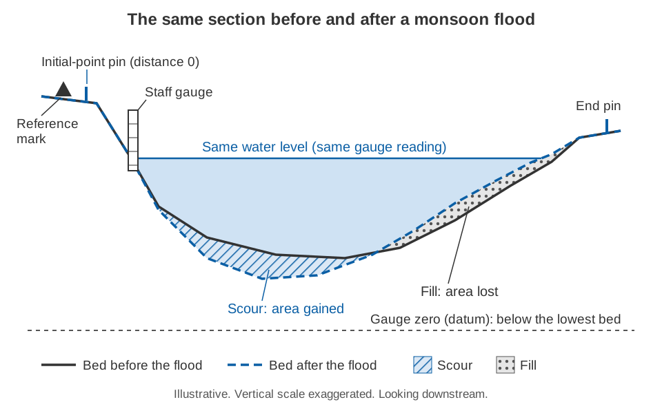
A flood does not just pass through a section; it rebuilds it. The WMO Manual advises looking for evidence of scour and deposition in past floods when choosing a gauging site, as a guide to what future floods will do [1].
In gravel-bed rivers the bed is mobile in floods and the change is patchy. Haschenburger measured scour and fill with scour chains in six gravel-bed channels 6 to 20 m wide. The depths followed an exponential distribution: many places changed a little and a few changed a lot. Estimating the mean depth to within 10 % at 95 % confidence needed more than 400 observations [6]. A few spot soundings cannot show how a section has changed; a full profile is needed.
In the Himalaya the changes can be extreme. On 15 June 2021 a high-concentration flow on the Melamchi and Indrawati rivers in central Nepal raised the channel bed by up to 12 m along a reach of about 30 km, while the neighbouring Bhote Koshi was largely unaffected [9]. At the everyday end of the scale, a study of three lesser Himalayan headwater streams (the Aglar, Paligaad and Balganga) found substantial inconsistency in the stage-discharge relation, especially at high flows. Its authors noted that alternating scour and fill, with deposition in the dry season and erosion and redeposition in the rains, can change a channel's conveyance [10].
The stage record is affected too. The CWC manual covers the case where scour drops the river below the lowest staff gauge while flow continues: the observer records a negative stage, and the engineer in charge re-surveys the station and reinstalls the gauges with a new, fully documented datum [5]. The WMO Manual likewise allows the gauge datum to be changed after excessive scour, preferably in whole metres so that old and new records can be related [1].
How a cross-section is surveyed
The aim is a list of points, each with a horizontal distance from a fixed initial point on the bank and a bed elevation in the gauge datum. Several methods are used, often together.
Banks and shallow water: level, staff and total station
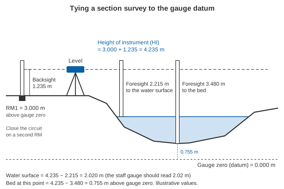
On the banks and in shallow water, the bed is surveyed with an engineer's level and a graduated staff. A backsight on a staff held on a reference mark of known elevation gives the height of instrument; each foresight on the staff held at a bed point is subtracted from it to give that point's elevation. A total station, an electronic instrument that measures angles and distances together, records position and elevation in one step. The WMO Manual recommends it for surveying reaches because it combines vertical and horizontal control in one operation [1].
Wading: rod and tag line
In wadeable water a tag line is stretched from the initial point and depth is read on a wading rod at each station, to the nearest 0.01 ft (about 3 mm) in USGS practice. On soft beds the rod's foot can sink, and water piling up against the rod in fast flow should not be read as depth [3]. Bed elevation is the water-surface elevation minus depth, so the water surface must be levelled or read on the gauge during the survey.
Deep water: sounding weights and echo sounders
From a bridge, cableway or boat, depth is measured with a sounding weight on a cable. In deep, fast water the weight is swept downstream and the cable leans, so the cable paid out exceeds the true depth and air-line and wet-line corrections are needed [1][3]. A sonic sounder (echo sounder) measures depth acoustically; the one described in the WMO Manual reaches 80 m. Temperature affects the speed of sound by up to about ±2 % in fresh water, an error removed by adjusting the sounder to a known depth. It suits swift, debris-laden water where lowering a weight is dangerous [1].
Boats: ADCP and satellite positioning
An acoustic Doppler current profiler (ADCP) on a moving boat measures depth on each of its four beams as well as velocity, so every transect also records a bed profile [1]. Its track across the river normally comes from bottom tracking, the Doppler shift of echoes from the bed [1]. Where the bed itself is moving, as in a gravel-bed river in flood, bottom tracking is biased, and the USGS manual refers to differentially corrected satellite positioning (DGPS) or the loop method instead. Uncorrected positions can be in error by as much as ±300 ft (about 90 m), reduced to about ±3 ft (1 m) or less with differential corrections, and trees, buildings and bridges can block or reflect the signals [3]. Whatever the method, the survey must still be tied to the station's reference marks.
Tying the section to the gauge datum
A section survey is useful only if it shares a datum with the gauge. The gauge datum is the level of the gauge's zero, kept permanent for the life of the station and protected by at least three reference marks (RMs) independent of the gauge structure [1]. How the datum is chosen and tied to the national datum, and what goes wrong when records use different zeros, is explained in gauge zero, datum and benchmarks.
In practice:
- Set permanent initial-point and end pins on both banks; a standard cross-section is useful only if every measurement uses the same initial point [1].
- Start from one RM and close the levelling circuit on another. The USGS standard is at least two foresights from different instrument heights to at least two independent RMs, with a closure error of no more than 0.003 ft (about 0.9 mm) per instrument setup and never more than 0.015 ft (about 4.6 mm) [4].
- Level the water surface and staff gauge in the same circuit, to check the gauge.
- While the level is set up, survey the control, bank-full level and any fresh high-water marks. A section of the control in gauge datum is easy to obtain during a level run and helps in developing the rating [4].
How often to re-survey
No single interval suits every river, but the manuals point to three triggers: a schedule, a flood, and evidence from the gaugings.
| Source | What it says |
|---|---|
| CWC field manual [5] | Re-survey float-gauging reach sections at least once a year, before the monsoon, and prepare new area tables after each re-survey. Check slope-area sections at least once a year, between monsoon seasons. If scour takes the river below the gauges, re-survey and reset the datum. |
| WMO Manual, site survey [1] | Survey the section more than once and compare for bed and bank stability, including immediately after a significant flood. Ideally build a history over several years, with one survey before and one immediately after the high-flow season. |
| WMO Manual, levels [1] | Run levels to gauges and RMs at least once a year at new sites and where the datum is not stable; every 2 or 3 years once it is fairly stable. |
| USGS levels manual [4] | Three annual sets in the first three years, then every 3 years, or every 5 years once stability is shown over at least 10 years. Run levels whenever flood damage or other disturbance is suspected. |
| USGS gauging manual [3] | When measuring a flood from pre-determined bed elevations, determine them again after the flood recedes to see whether they changed. |
The WMO site-survey advice comes from its chapter on acoustic velocity stations, but applies to any station that relies on a section. For a gravel-bed river in India, a practical reading is:
- Before every monsoon, survey the measuring section and the control, and run levels to the gauge and RMs.
- After every flood large enough to move the bed, re-survey as soon as it is safe, even if the scheduled survey is months away.
- Whenever gaugings drift from the current rating, consistently on one side, survey the section and the control before fitting a new curve.
- Keep every survey with its date and never overwrite an old one. Discharge for each period should be computed with the section that was valid then.
The last two points are where research has helped most. Mansanarez and colleagues treat the record as a series of stability periods separated by known dates of change, such as floods, and estimate all the rating curves together by Bayesian inference. Information carries across periods, and the curves come out more precisely than when each period is fitted separately [7]. A dated post-flood survey supplies exactly those dates. Ignoring change is costly. On the alluvial Choluteca River in Honduras, where fill and scour make the stage-discharge relation non-stationary, a time-varying rating differed from a single constant one by −60 to +90 % at low flows and ±20 % at medium to high flows [8].
Key points
- Discharge from a rating curve or from area × velocity is only as good as the cross-section behind it.
- In the illustrative 30 m channel, 0.3 m of fill made the old rating over-read by 30 % and velocity-area with the old area by 18 %; 0.3 m of scour gave −20 % and −13 %.
- Floods change gravel-bed and Himalayan river beds unevenly, so survey a full profile.
- Use level and staff or total station on the banks, a rod when wading, weights or echo sounder in deep water, and ADCP with satellite positioning from boats.
- Tie every survey to the gauge datum through permanent reference marks and pins, and close the levelling circuit.
- Re-survey before each monsoon, after each bed-moving flood and whenever gaugings drift from the rating, and keep every dated version.
At ClimMaTech we work on river stations in Himalayan catchments, where the riverbed is rarely the one surveyed last season. See PRAVAAH, an AWLR and surface velocity radar (SVR) that gives non-contact discharge from a surveyed cross-section and a site-calibrated surface coefficient, and our river monitoring solutions, and can radar measure river discharge? for how level and velocity records relate to discharge.
References
- World Meteorological Organization, Manual on Stream Gauging, Volume I: Fieldwork, WMO-No. 1044, WMO, 2010, Chapters 2 to 6 and 9. wmo.int (PDF).
- International Organization for Standardization, ISO 748:2021 Hydrometry — Measurement of liquid flow in open channels — Velocity area methods using point velocity measurements, ISO, 2021. iso.org.
- D. P. Turnipseed and V. B. Sauer, Discharge Measurements at Gaging Stations, U.S. Geological Survey Techniques and Methods, book 3, chapter A8, 2010. doi.org/10.3133/tm3A8.
- T. A. Kenney, Levels at Gaging Stations, U.S. Geological Survey Techniques and Methods, book 3, chapter A19, 2010. doi.org/10.3133/tm3A19.
- Central Water Commission, Gauge & Discharge Measurement Field Manual, Volume 4 Hydrometry, Parts II, III, IV and VI, River Data Directorate, CWC, January 2005. cwc.gov.in (PDF).
- J. K. Haschenburger, A probability model of scour and fill depths in gravel-bed channels, Water Resources Research 35(9), 2857–2869, 1999. doi.org/10.1029/1999WR900153.
- V. Mansanarez, B. Renard, J. Le Coz, M. Lang and M. Darienzo, Shift happens! Adjusting stage-discharge rating curves to morphological changes at known times, Water Resources Research 55, 2876–2899, 2019. doi.org/10.1029/2018WR023389.
- I. Westerberg, J.-L. Guerrero, J. Seibert, K. J. Beven and S. Halldin, Stage-discharge uncertainty derived with a non-stationary rating curve in the Choluteca River, Honduras, Hydrological Processes 25, 603–613, 2011. doi.org/10.1002/hyp.7848.
- E. L. S. Graf, H. D. Sinclair, M. Attal, B. Gailleton, B. R. Adhikari and B. R. Baral, Geomorphological and hydrological controls on sediment export in earthquake-affected catchments in the Nepal Himalaya, Earth Surface Dynamics 12, 135–161, 2024. doi.org/10.5194/esurf-12-135-2024.
- V. Kumar and S. Sen, Rating curve development and uncertainty analysis in mountainous watersheds for informed hydrology and resource management, Frontiers in Water 5, 1323139, 2024. doi.org/10.3389/frwa.2023.1323139.