Data assimilation in flood forecasting, simply explained

A flood model is started in the morning with a forecast that the river at a town will peak at 4.2 m by evening. By noon the gauge already reads 4.5 m and is still rising. The model did not know about the heavier rain upstream or the wetter soil. A forecaster has two options: trust the model and ignore the gauge, or use the gauge to correct the model. Data assimilation is the second option made systematic. This article explains the data assimilation meaning in hydrology, the main methods including the ensemble Kalman filter, and what these methods can and cannot do for a flood warning.

What is data assimilation, in plain words?

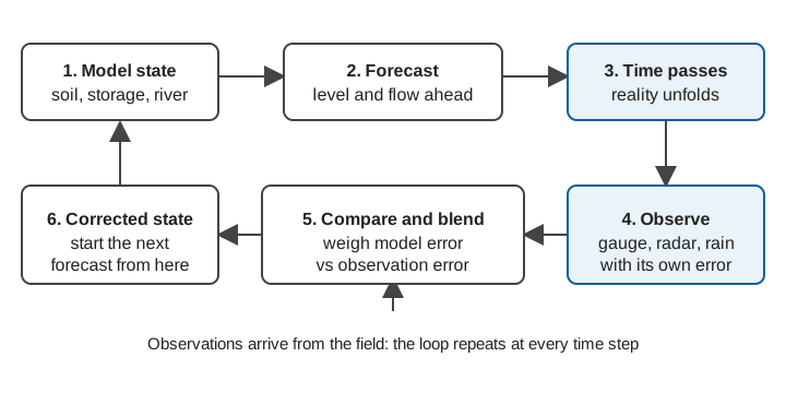
Data assimilation is the process of feeding new observations into a running model so that its internal picture of the catchment, and therefore its forecast, moves closer to reality. The model carries the physics; the observations carry the truth, with some noise. Assimilation weighs one against the other by how far each can be trusted.

The WMO Manual on Flood Forecasting and Warning (WMO-No. 1072) puts the aim simply: in real-time flood forecasting a large number of observations are collected, and the scope of data assimilation is "the incorporation of this information into the model state variables or into the model parameters to improve the forecasting performances" [1].

Two terms need defining before going further:

• State: the model's current internal condition, such as how much water is stored in the soil, in a groundwater store, and in each river reach. The state is what the model carries forward from one time step to the next.
• Parameter: a model constant, such as a runoff coefficient or a channel roughness, that is set by calibration and normally stays fixed.

Forecast error comes from the weather input, the state, the parameters and the observations themselves; the WMO manual notes that errors in spatially averaged rainfall alone "can easily be between 20 and 30 per cent" [1].

Why forecasts need correcting while a flood is happening

Simulating a past flood and forecasting the next few hours are different jobs. The WMO manual says a model run without updating "ignores the availability of the sequence of observed flows up to the time origin of the forecast" and "inevitably leads to the simulated forecasts drifting further away from the subsequently observed flow values" [1].

It also describes the three ways a simulated flood hydrograph can be wrong: amplitude errors (the volume or peak is too high or low), phase errors (the timing is early or late) and shape errors (both) [1]. Updating aims to reduce all three.

What are the main ways of updating a flood forecast?

There is no single method. The WMO manual notes that updating procedures "differ in detail or in their mode of operation" but all provide the model with feedback from recently observed flows to estimate errors and improve accuracy [1]. The review by Liu and colleagues groups the work into several kinds [2]; three matter most for flood forecasting.

Output (error) correction

The simplest approach leaves the model alone and corrects its answer. If the model has been under-predicting by 0.30 m at the gauge for the last few hours, add a decaying correction to the forecast. Liu et al. describe operational versions that fit a time-series model to the recent forecast errors and project them forward [2]. It is cheap and robust, but it only fixes the output; the model's state stays wrong, so the benefit fades with lead time.

The WMO manual makes the same point: an efficient updating procedure "can substantially improve the accuracy of the forecasts for short lead times", whereas at longer lead times improvement "can be achieved only through the improvement of the simulation-mode forecasts" [1].

State updating

Here the internal state of the model is adjusted. If the gauge is higher than expected, perhaps the soil store was wetter than the model thought. Changing those stores makes the model's own physics carry the correction forward, so later forecast hours are affected consistently, not just the first few. This is the type of assimilation the Kalman filter family performs [2][3].

Parameter updating

Parameters can also be adjusted, at every step or by periodic recalibration. The WMO manual cautions that such "adaptive calibration" is hard to justify physically given the quality of data generally available, and "extremely difficult" for complex or distributed models [1]. Joint estimation of states and parameters has been explored with the ensemble Kalman filter, for example by Moradkhani and co-authors with a conceptual rainfall-runoff model [4].

How does the Kalman filter work?

The Kalman filter blends a forecast and an observation in proportion to how uncertain each is. The WMO manual presents it as the recursive method that finds the best estimate of the state given the previous estimate, its error covariance and the latest noisy measurement, written in terms of a Kalman gain [1]. For a single variable, it reduces to:

analysis = forecast + K × (observation − forecast)

K = forecast variance / (forecast variance + observation variance)
analysis variance = (1 − K) × forecast variance

The bracketed difference is the innovation: how far the observation is from what the model expected. The gain K lies between 0 and 1. If the observation is very precise, K approaches 1 and the model is pulled towards the gauge. If the observation is noisy, K approaches 0 and the model is left mostly alone.

A worked example (illustrative)

Take the stage forecast from the opening. The model says 4.20 m, with an uncertainty (standard deviation) of 0.30 m. The gauge reads 4.50 m, with an assumed uncertainty of 0.10 m in the reading under flood conditions.

forecast variance    = 0.30² = 0.090 m²
observation variance = 0.10² = 0.010 m²
K        = 0.090 / (0.090 + 0.010) = 0.90
analysis = 4.20 + 0.90 × (4.50 − 4.20) = 4.47 m
analysis variance = (1 − 0.90) × 0.090 = 0.009 m²  → sd ≈ 0.095 m

The result, 4.47 m, sits close to the gauge because the gauge is more precise than the model. Its uncertainty (0.095 m) is smaller than either input. Had the gauge uncertainty been 0.30 m, K would be 0.5 and the answer would sit halfway, at 4.35 m. This is why knowing the uncertainty of observations matters; see measurement uncertainty for water data and rating curves and their uncertainty, since a discharge "observation" derived from a rating curve is itself a model output.

A river model has thousands of state variables, not one, and the original Kalman filter assumes a linear model. The extended Kalman filter linearises the model locally, but Liu et al. note that the linearisation can be unrealistic and the derivatives difficult to compute reliably, so it "has fallen out of favour" [2].

What is the ensemble Kalman filter?

The ensemble Kalman filter (EnKF) replaces the algebra of error covariances with a crowd of model runs. Introduced by Geir Evensen in 1994, it was set out in full, with its practical implementation, in his 2003 paper [3]. Evensen credits its popularity to its "simple conceptual formulation and relative ease of implementation": it needs no linearised model and no run backwards in time [3].

The procedure is:

1. Run the model many times (the ensemble), each member with slightly different inputs, states or parameters, to represent the uncertainty.
2. When an observation arrives, compare it with each member's prediction of that observation, with a little random noise added to the observation for each member.
3. Move each member towards the observation by an amount set by a gain calculated from the spread of the ensemble itself.
4. Continue forecasting from the updated members.

Liu et al. report that the EnKF "has become the most frequently used DA technique in the hydrologic community, due largely to its easy implementation and its robustness" [2]. Evensen shows that for linear models it converges to the Kalman filter as the ensemble size grows without limit [3].

The same example with an ensemble (illustrative)

Suppose five members forecast discharge at a gauge as 180, 210, 240, 270 and 300 m³/s, and the observation is 300 m³/s with an uncertainty of 20 m³/s.

ensemble mean        = 240 m³/s
ensemble variance    = (60² + 30² + 0 + 30² + 60²) / 4 = 2250  (sd ≈ 47 m³/s)
observation variance = 20² = 400
K                = 2250 / (2250 + 400) = 0.85
mean after update = 240 + 0.85 × (300 − 240) ≈ 291 m³/s
variance after    = (1 − 0.85) × 2250 ≈ 340  (sd ≈ 18 m³/s)

The mean moves most of the way to the observation and the spread tightens. Real systems use far more members: Liu et al. note that "typically, hundreds of ensemble members" are needed for reliable updating without filter inbreeding[2].

What are the limits of data assimilation?

Assimilation helps a good model; it does not replace one. Liu et al. state that advances in research "have not been adequately or timely implemented in operational forecast systems", partly because of the difficulty of quantifying uncertainty in observations and models in real time, and of merging data and models "in a way that is adequately efficient and transparent to operational forecasters" [2]. Among the practical limits:

• Wrong uncertainties give wrong weights. If the observation error is understated, the filter chases a faulty reading. Data quality control comes first; see quality control for hydromet time series.
• Gaussian assumptions. The EnKF performs best when states and parameters are roughly Gaussian (bell-shaped) [2]. Flows, which cannot be negative and are skewed, may need transformations or other methods such as the particle filter [2].
• Bias. Updating assumes errors are random. Liu et al. note that systematic or time-varying bias must be removed as far as possible [2]; a stage-gauge datum offset is a typical example.
• Sparse networks. The update can only be as good as the observations. In steep Himalayan catchments, where a flood wave can reach a town within hours, a single upstream gauge may be the only information available; see flash floods versus river floods and river monitoring in hill catchments.

For the rainfall side of the ensemble idea, see ensemble weather forecasts; for the models themselves, hydrological models explained and machine learning for flood forecasting.

Key points

• Data assimilation uses live observations to correct a running model's state, parameters or output, so that forecasts start from where the river actually is.
• Output correction is the simplest method; state updating makes the model's physics carry the correction forward.
• The Kalman filter weights model and observation by their uncertainties; the ensemble Kalman filter estimates those uncertainties from a set of model runs and is the most used method in hydrology.
• The benefit is largest at short lead times and fades with lead time; it cannot rescue a poor model or a poor rainfall forecast.
• All of it depends on timely, quality-controlled observations with known uncertainty.

Where ClimMaTech fits

Assimilation works only where there are trustworthy, frequent observations to assimilate. At ClimMaTech we build the observing end of that chain: Tarang is an AWLR (Automatic Water Level Recorder) with a radar level sensor accurate to ±1 mm under ideal conditions, and PRAVAAH adds a Surface Velocity Radar (SVR) so a river section reports level and surface velocity together. Observations like these, with documented uncertainty, are what a forecaster or a model needs, and our flood warning solution page describes how they connect to warning dissemination.

References

1. World Meteorological Organization, Manual on Flood Forecasting and Warning, WMO-No. 1072, 2011 edition, sections 3.2.3, 3.2.6 and 4.6. old.wmo.int (PDF)
2. Y. Liu, A. H. Weerts, M. Clark, H.-J. Hendricks Franssen, S. Kumar, H. Moradkhani, D.-J. Seo, D. Schwanenberg, P. Smith, A. I. J. M. van Dijk, N. van Velzen, M. He, H. Lee, S. J. Noh, O. Rakovec, P. Restrepo, Advancing data assimilation in operational hydrologic forecasting: progresses, challenges, and emerging opportunities, Hydrology and Earth System Sciences 16, 3863–3887, 2012. doi:10.5194/hess-16-3863-2012
3. G. Evensen, The Ensemble Kalman Filter: theoretical formulation and practical implementation, Ocean Dynamics 53, 343-367, 2003. doi:10.1007/s10236-003-0036-9
4. H. Moradkhani, S. Sorooshian, H. V. Gupta, P. R. Houser, Dual state-parameter estimation of hydrological models using ensemble Kalman filter, Advances in Water Resources 28(2), 135–147, 2005. doi:10.1016/j.advwatres.2004.09.002