
Types of hydrological models: rainfall-runoff to hydraulics
How hydrological and hydraulic models are classified, what each kind can and cannot do, how they are calibrated and scored, and why every one of them depends on good river and rainfall data.

Every flood forecast and design flood rests on a model, yet "the model" is often a black box to the people who use its numbers. A district officer reading tomorrow's forecast level, or an engineer checking a consultant's design flood, can judge that number better if they know what kind of model produced it. This article explains the main types of hydrological models, how they differ from hydraulic models, how they are calibrated and scored, and what they need from the monitoring network.
What is a hydrological model?
A hydrological model is a set of equations that turns inputs such as rainfall, snowmelt and evaporation into outputs such as river discharge (the volume of water passing a point per second, in m³/s). The commonest kind, the rainfall-runoff model, answers two questions: how much of the rain becomes river flow, and when does it arrive? Beven's standard text describes the field as predicting hydrographs "using models based on data and on representations of hydrological process" [1]. A hydrograph is a graph of discharge against time (see what a hydrograph tells you). The catchment itself is delineated first, as explained in catchments and watersheds.
What are the types of hydrological models?
Hydrological models are classified in three independent ways: by how they describe the physical processes, by how they divide the catchment in space, and by how they handle time. The WMO Manual on Flood Forecasting and Warning (WMO-No. 1072) uses the same distinctions [2].
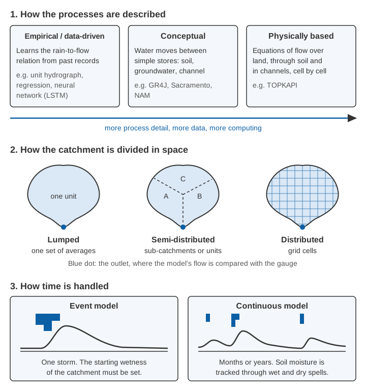
By process: empirical, conceptual or physically based
- Empirical or data-driven models learn the input-output relation from past records without describing the physics: the unit hydrograph, regression on upstream levels, neural networks. WMO calls them "generally simple and easy to calibrate", but notes that users fear they are less reliable beyond the range of their data, and recommends them for gauged sites with long records [2].
- Conceptual models represent the catchment as a few connected stores (soil, groundwater, channel) with water moving between them by simple rules. Their parameters are adjusted until the model matches observed flow. WMO calls them "the most widely used for flood forecasting", partly because flood managers find them easy to understand [2]. GR4J, a daily model with four parameters, is an example [3].
- Physically based models solve the equations of water movement over land, through soil and in channels, usually cell by cell. WMO recommends them where terrain and soil data are good, where forecasts are needed at ungauged places, and where rainfall varies strongly and is available as a grid, for example from radar [2].
By space: lumped, semi-distributed or distributed
A lumped model treats the whole catchment as one unit with average rainfall and one set of parameters. A semi-distributed model runs sub-catchments or response units separately. A distributed model works on a grid of cells [2].
What is a distributed hydrological model?
A distributed hydrological model calculates the water balance separately for many small cells across the catchment, so rainfall, soils, land use and slope can differ from place to place. WMO lists two advantages: it makes the best use of gridded rainfall from radar and weather models, and its parameters can keep their physical meaning for cells of a few square kilometres, which helps in ungauged catchments. Lumped models run faster. When the manual was written, most operational forecasting models were lumped models arranged as semi-distributed networks, and fully distributed models in real-time use were "still rare" [2].
The Variable Infiltration Capacity (VIC) model is a well-known grid-based example: each cell is split into land-cover types, and both the water and the energy balance of the land surface are computed [4]. SWAT (Soil and Water Assessment Tool) is a continuous model built for large river basins and land-management questions [5].
By time: event or continuous
An event model simulates one storm; a continuous model runs through months or years and tracks soil moisture between storms. The catch with event models is the starting state: without a "warm-up period" the initial conditions must be guessed, which makes event modelling subjective, so WMO restricts them to cases where the initial state is known, such as floods that always come when the soil is already wet [2]. In much of India that fits the peak of the monsoon, not its first storms. WMO cites HEC-HMS, free software from the US Army Corps of Engineers, as a popular event model [2]. Design studies use event models with a design storm, often from IDF curves.
Data-driven and machine-learning models
A long short-term memory (LSTM) network is a neural network that keeps a memory of past inputs, which suits catchments where today's flow depends on weeks of earlier rain. Trained on 531 basins at once, a single LSTM did better than benchmark hydrological models calibrated basin by basin [6]. For extreme floods in ungauged watersheds, an AI-based system forecasting up to five days ahead matched or beat the same-day estimates of an established global flood forecasting system, and now runs operationally in over 80 countries [7].
In our comparison of SWAT and GR4J with random forest, neural network and LSTM models, GR4J was marginally better than SWAT; random forest and a bidirectional LSTM captured extreme flows better, the process-based models suited medium flows, and the choice of inputs made a marked difference [3]. Across 144 watersheds in the Indian subcontinent, our best deep-learning model reached a median Nash–Sutcliffe efficiency of 0.71 on test basins, from 0.849 in tropical monsoon regions to 0.586 in semi-arid ones. Because it needed recent observed streamflow, we built a second network that matches its skill without it, for ungauged basins [8].
WMO's caution still applies: a model that learnt from the past is least reliable beyond the range of its data [2]. Machine learning has not removed the need for long, good-quality records. It has increased it.
What is the difference between hydrologic and hydraulic modelling?
Hydrologic modelling estimates how much water reaches the river and when; hydraulic modelling calculates how that water flows along the channel and over the floodplain, giving water level, velocity and flooded area. In a forecasting chain the hydrological model's discharge becomes the hydraulic model's input.
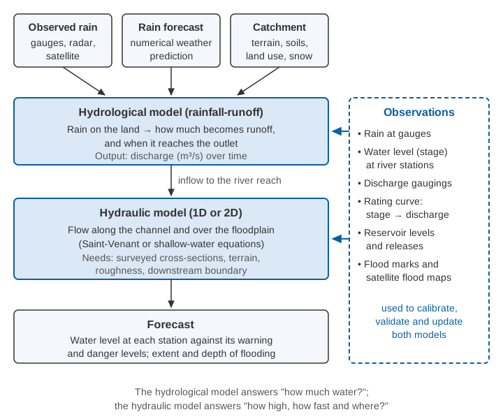
Most hydraulic models of rivers solve the Saint-Venant equations, which express conservation of mass and momentum for flow along a channel. In the form given in WMO-No. 1072 [2]:
Continuity:  ∂y/∂t + D·∂V/∂x + V·∂y/∂x = q
Momentum:    Sf = S0 − ∂y/∂x − (V/g)·∂V/∂x − (1/g)·∂V/∂t

y  = flow depth (m)              V  = mean velocity (m/s)
D  = hydraulic depth (m)         q  = lateral inflow
x  = distance along river (m)    t  = time (s)
S0 = bed slope                   Sf = friction slope
g  = acceleration due to gravity (9.81 m/s²)
They assume one-dimensional flow, hydrostatic pressure, a fixed bed and a small slope, among other conditions [2]. Solving the full set (dynamic routing) is needed for rapidly varying flows such as a dam breach; for ordinary routing the simpler kinematic wave (Sf = S0) and diffusion wave (adding the water-surface gradient) are widely used [2]. Storage methods such as Muskingum are simpler still; see how a flood early warning system works.
One-dimensional (1D) models describe the river as a series of surveyed cross-sections, so they need up-to-date cross-section surveys. Bangladesh's flood forecasting centre, for example, linked a 1D hydrodynamic model of its major rivers (MIKE 11 HD) to a lumped conceptual rainfall-runoff model supplying inflows from secondary catchments [2]. Two-dimensional (2D) models solve the shallow-water equations over a grid or mesh of the floodplain, showing where water spreads once it leaves the channel; they are demanding enough to compute that efficient formulations are a research topic of their own [9]. A study of the 2006 Surat flood coupled both in HEC-RAS: 299 cross-sections in the 1D river model, a 5 m grid of the city in 2D, the Ukai Dam release as the upstream boundary and the tide as the downstream one. It found 75–77 % of the city inundated on the worst day [10].
How are models calibrated and validated?
Calibration means adjusting a model's parameters until its output matches observations; validation means testing it on a period it has not seen. The classic split-sample test divides the record in two. Klemeš warned that even a fully successful test is a necessary, not a sufficient, condition for a model to be adequate [11]. WMO recommends a verification period ideally as long as the calibration period and long enough to include several floods, often two years or more [2].
Two scores dominate:
Nash–Sutcliffe efficiency:  NSE = 1 − Σ(Qsim − Qobs)² / Σ(Qobs − mean Qobs)²

Kling–Gupta efficiency:     KGE = 1 − √[(r − 1)² + (α − 1)² + (β − 1)²]
   r = correlation between simulated and observed flow (timing and shape)
   α = σsim / σobs   (ratio of standard deviations: variability)
   β = μsim / μobs   (ratio of means: bias in volume)
NSE comes from Nash and Sutcliffe [12]. A perfect model scores 1; NSE = 0 means the model is no better than the mean observed flow [13]. Gupta and colleagues showed that calibration based on NSE or mean squared error has systematic problems and proposed KGE, which keeps correlation, variability and bias separate [14]. KGE is also 1 for a perfect model, but the mean flow scores about −0.41, not 0, so the two scores are not directly comparable [13].
Worked example: two models, one flood
The numbers below are illustrative. Six daily flows were observed during a small flood, and two calibrated models simulated them:
| Day | Observed (m³/s) | Model A | Model B |
|---|---|---|---|
| 1 | 20 | 24 | 30 |
| 2 | 60 | 50 | 70 |
| 3 | 140 | 120 | 110 |
| 4 | 100 | 110 | 100 |
| 5 | 60 | 70 | 70 |
| 6 | 40 | 46 | 50 |
NSE for Model A. The observed mean is 420 / 6 = 70 m³/s. The errors are 4, −10, −20, 10, 10 and 6, whose squares sum to 16 + 100 + 400 + 100 + 100 + 36 = 752. The observed deviations from the mean are −50, −10, 70, 30, −10 and −30, whose squares sum to 2,500 + 100 + 4,900 + 900 + 100 + 900 = 9,400. So NSE = 1 − 752 / 9,400 = 0.92.
KGE for Model A. The simulated mean is also 70, so β = 1. The standard deviations are √(9,400 / 6) = 39.6 m³/s observed and √(7,192 / 6) = 34.6 m³/s simulated, so α = 34.6 / 39.6 = 0.875. The correlation is r = 0.963. Then KGE = 1 − √[(0.963 − 1)² + (0.875 − 1)² + 0] = 1 − √0.0170 = 0.87.
Model B, by the same arithmetic: squared errors sum to 1,300, so NSE = 1 − 1,300 / 9,400 = 0.86, but α = 0.69, r = 0.970 and β = 1.02, so KGE = 0.69.
On NSE the two models look similar. KGE marks Model B down because it smooths the flood and its peak is 21 % low, exactly the error that matters for a warning. Always look at the hydrograph, peak and volume too.
Try calibrating a model
The toy model below combines two classic pieces. The NRCS curve number method estimates how much of the rain becomes direct runoff, using a curve number CN between 0 and 100: the higher the number, the more of the rain runs off. The NRCS adjusts CN for how wet the catchment is before the storm [15]. A linear reservoir, in which outflow is proportional to storage, then spreads that runoff over time. Move the sliders to fit the observed hydrograph.
The figures are illustrative. The "observed" hydrograph is synthetic, generated for this example with a slightly different model structure.
Three lessons follow. CN sets the volume and K the timing, but they interact, and several combinations score similarly. The best NSE (about 0.93, near CN 79, K 6 h) and the best KGE (about 0.94, near CN 78, K 4.5 h) come from different parameter sets, so the choice of score changes the "calibrated" model. And no setting makes the model rise as late and as steeply as the observations, because the real flow passed through more storage than one reservoir represents. That is structural error, and calibration cannot remove it.
Where does model uncertainty come from?
Model uncertainty comes from four sources: inputs, the observations used for calibration, parameters and model structure [2]. WMO notes that errors in spatially averaged rainfall "can easily be between 20 and 30 per cent", and that measured levels and discharges can be biased by instrument errors [2]. Different parameter sets of one model can give almost equal efficiency, so WMO describes systems that combine several models or parameter sets rather than trusting one [2].
Uncertainty also cascades. One European study passed 52 rainfall forecasts through a rainfall-runoff model with six parameter sets, then an inundation model with ten roughness sets; a full analysis was limited mainly by computing power and by the quality of the rainfall forecasts [16]. See also measurement uncertainty in plain language.
What models need from observations
Every model is only as good as the data it is built on and checked against:
- Rainfall at adequate density and time step; see how many rain gauges a district needs.
- Water level (stage) at river stations, continuous and tied to a stable datum. Hydraulic models are checked against it.
- Discharge, almost always derived from level through a rating curve. WMO insists on "the most up-to-date rating relationship", notes that mobile-bed rivers need frequent gaugings, and warns that a changed rating may mean recalibrating the model [2]; see rating curves and their uncertainty.
- Clean records, because spikes, gaps and drift become errors in the parameters; see data quality control.
When results look wrong, WMO advises against recalibrating for a better fit and asks modellers "to carefully investigate the cause from both sides, observation and modelling" [2].
Ungauged catchments can borrow parameters from similar gauged "donor" catchments, a technique called regionalisation. In our study of ten catchments, grouping them by both physical and climatic attributes gave the best GR4J parameter transfer [17]. Donors still have to be gauged: regionalisation spreads the value of a good station; it does not replace it.
Which hydrological model is used for flood forecasting?
No single model is best for flood forecasting: WMO states that "there is no specific type of model that can be chosen as the most appropriate", and that purpose and available data should decide [2]. It compares the lead time needed with the catchment's time of concentration or travel time: data-driven methods suit lead times that are short relative to it, conceptual models lead times of the same order. A forecast must also be robust and on time, which can rule out slow, sophisticated models [2].
India's Central Water Commission (CWC) layers several methods. Its Standard Operating Procedure of April 2025 lists 340 forecasting stations, 200 for river level and 140 for inflow to dams and barrages, and more than 8,000 forecasts a season [18]. Short-range forecasts of 6 to 24 hours use statistical methods such as correlation curves and unit hydrographs; a rainfall-runoff-model advisory, 3 days in 2017 and 5 days from 2021, has covered 7 days since 2023 [18]. A level forecast counts as accurate within ±15 cm, an inflow forecast within ±20 %, and 1,121 telemetry stations supply water level and rainfall [18]. The model sits in the middle of the chain; the gauges feed it and judge it.
Key points
- Models are classified by process (data-driven, conceptual, physically based), space (lumped, semi-distributed, distributed) and time (event, continuous).
- Hydrological models turn rain into discharge; hydraulic models turn discharge into levels, velocities and flood extent.
- Machine-learning models perform strongly in large tests, including Indian basins, but are least reliable beyond their training data.
- Validate on data the model has not seen, and use more than one score: NSE and KGE reward different things.
- Uncertainty comes from inputs, observations, parameters and structure, and cascades along the chain.
- Every model depends on long, clean records of rainfall, level and discharge, with an up-to-date rating curve.
Where ClimMaTech fits
Our team's research includes hydrological and machine-learning modelling, as in the studies cited above, and our monitoring work sits at the observation end of the chain. Continuous water level and surface velocity from PRAVAAH give models observations to be calibrated, checked and updated against, and our flood warning page describes how upstream readings, thresholds and an authorised operator turn into warnings on the ground.
References
- K. J. Beven, Rainfall-Runoff Modelling: The Primer, 2nd edition, Wiley-Blackwell, 2012. doi:10.1002/9781119951001
- World Meteorological Organization, Manual on Flood Forecasting and Warning, WMO-No. 1072, WMO, 2011 (sections 3.2–3.4, 4.1, 4.3–4.5). WMO PDF
- S. Barbhuiya, A. Manekar, M. Ramadas, Performance evaluation of ML techniques in hydrologic studies: Comparing streamflow simulated by SWAT, GR4J, and state-of-the-art ML-based models, Journal of Earth System Science 133, 136, 2024. doi:10.1007/s12040-024-02340-0
- X. Liang, D. P. Lettenmaier, E. F. Wood, S. J. Burges, A simple hydrologically based model of land surface water and energy fluxes for general circulation models, Journal of Geophysical Research: Atmospheres 99(D7), 14415–14428, 1994. doi:10.1029/94JD00483
- J. G. Arnold, R. Srinivasan, R. S. Muttiah, J. R. Williams, Large area hydrologic modeling and assessment part I: Model development, Journal of the American Water Resources Association 34(1), 73–89, 1998. doi:10.1111/j.1752-1688.1998.tb05961.x
- F. Kratzert, D. Klotz, G. Shalev, G. Klambauer, S. Hochreiter, G. Nearing, Towards learning universal, regional, and local hydrological behaviors via machine learning applied to large-sample datasets, Hydrology and Earth System Sciences 23, 5089–5110, 2019. doi:10.5194/hess-23-5089-2019
- G. Nearing, D. Cohen, V. Dube, M. Gauch, O. Gilon, S. Harrigan, A. Hassidim, D. Klotz, F. Kratzert, A. Metzger, S. Nevo, F. Pappenberger, C. Prudhomme, G. Shalev, S. Shenzis, T. Y. Tekalign, D. Weitzner, Y. Matias, Global prediction of extreme floods in ungauged watersheds, Nature 627, 559–563, 2024. doi:10.1038/s41586-024-07145-1
- S. Barbhuiya, V. Gupta, From gauged to ungauged: Large-scale deep learning rainfall-runoff modelling for reliable streamflow estimation in India's diverse basins, Environmental Modelling & Software 194, 106696, 2025. doi:10.1016/j.envsoft.2025.106696
- P. D. Bates, M. S. Horritt, T. J. Fewtrell, A simple inertial formulation of the shallow water equations for efficient two-dimensional flood inundation modelling, Journal of Hydrology 387(1–2), 33–45, 2010. doi:10.1016/j.jhydrol.2010.03.027
- D. Patel, J. Ramirez, P. K. Srivastava, M. Bray, D. Han, Assessment of flood inundation mapping of Surat city by coupled 1D/2D hydrodynamic modeling: a case application of the new HEC-RAS 5, Natural Hazards 89, 93–130, 2017. doi:10.1007/s11069-017-2956-6
- V. Klemeš, Operational testing of hydrological simulation models, Hydrological Sciences Journal 31(1), 13–24, 1986. doi:10.1080/02626668609491024
- J. E. Nash, J. V. Sutcliffe, River flow forecasting through conceptual models part I — A discussion of principles, Journal of Hydrology 10(3), 282–290, 1970. doi:10.1016/0022-1694(70)90255-690255-6)
- W. J. M. Knoben, J. E. Freer, R. A. Woods, Technical note: Inherent benchmark or not? Comparing Nash–Sutcliffe and Kling–Gupta efficiency scores, Hydrology and Earth System Sciences 23, 4323–4331, 2019. doi:10.5194/hess-23-4323-2019
- H. V. Gupta, H. Kling, K. K. Yilmaz, G. F. Martinez, Decomposition of the mean squared error and NSE performance criteria: Implications for improving hydrological modelling, Journal of Hydrology 377(1–2), 80–91, 2009. doi:10.1016/j.jhydrol.2009.08.003
- United States Department of Agriculture, Natural Resources Conservation Service, National Engineering Handbook, Part 630 Hydrology, Chapter 10: Estimation of Direct Runoff from Storm Rainfall, 210-VI-NEH, USDA NRCS, July 2004. directives.nrcs.usda.gov (PDF)
- F. Pappenberger, K. J. Beven, N. M. Hunter, P. D. Bates, B. T. Gouweleeuw, J. Thielen, A. P. J. de Roo, Cascading model uncertainty from medium range weather forecasts (10 days) through a rainfall-runoff model to flood inundation predictions within the European Flood Forecasting System (EFFS), Hydrology and Earth System Sciences 9, 381–393, 2005. doi:10.5194/hess-9-381-2005
- S. Barbhuiya, A. S. Raghuvanshi, H. L. Tiwari, Assessment of streamflow in ungauged basin by using physical similarity approach, Arabian Journal of Geosciences 16, 672, 2023. doi:10.1007/s12517-023-11786-3
- Central Water Commission, Ministry of Jal Shakti, Standard Operating Procedure for Flood Forecasting, CWC, April 2025 (sections 1.1, 1.4, 2.2 and 3.8). cwc.gov.in (PDF)