
Measurement uncertainty for water data, in plain language
What the ± after a water level or a discharge really means, how to work it out without heavy mathematics, and how to report it so that others can use your data with confidence.

A district engineer receives a report: discharge at the bridge was 72 m³/s at the peak. Is that 72 give or take 1, or give or take 20? The answer decides whether the number can be compared with last year's flood or fed into a model. Yet most hydrological records carry no such statement.
The Guide to the Expression of Uncertainty in Measurement, known as the GUM (JCGM 100:2008) [1], gives one method that works the same way for a laboratory balance and for a river. The hydrometric standards follow it: ISO 25377:2020, Hydrometric uncertainty guidance (HUG), applies it to flow measurement in natural and man-made channels [3], and the WMO Manual on Stream Gauging (WMO-No. 1044) devotes a chapter to it [4]. This article explains the method in plain language, then works through a discharge example step by step.
Error and uncertainty are not the same thing
The error of a measurement is the difference between the measured value and the true value. We can never know it exactly, because we never know the true value. The WMO Manual makes exactly this point: because the true discharge can never be known, the exact error in a discharge measurement can never be known either [4].
Uncertainty is what we can state. The GUM defines it as a parameter "that characterizes the dispersion of the values that could reasonably be attributed to the measurand" [1], where the measurand is the quantity we intend to measure (the discharge at this section at 14:00, say). In simple terms, uncertainty is an honest statement of how far the true value could plausibly be from our number.
A result can, by luck, be very close to the true value and still have a large uncertainty [1]. Uncertainty describes the quality of the method and information, not the luck of one reading.
- Systematic effects (bias) push every reading the same way, such as a wrongly set gauge zero. The GUM expects known biases to be corrected; what remains uncertain about the correction becomes one more uncertainty component [1].
- Random effects scatter readings both ways, such as turbulence making a velocity reading wander.
Agreement in pattern is not the same as small uncertainty. In our study comparing satellite rainfall with 32 rain gauges in the southern Himalaya of Bhutan over 19 years, the satellite series correlated well with the gauges (average correlation 0.814) yet underestimated rainfall, and its relative root-mean-square error exceeded 50 % at 96 % of stations, so we advised bias correction before use [8].
Two ways to evaluate an uncertainty: Type A and Type B
The GUM sorts evaluations by how the number is obtained, not by where the effect comes from [1]:
- Type A evaluation: by statistical analysis of repeated observations. Take ten surface-velocity readings, compute their standard deviation, and divide by the square root of the number of readings to get the uncertainty of the mean.
- Type B evaluation: by any other means. A calibration certificate, a manufacturer's specification, the stated accuracy of a survey, published values from earlier studies, or informed judgement.
Both are equally valid. The WMO Manual tabulates recommended component uncertainties for current-meter gaugings and notes that using them is a Type B evaluation, because they come from earlier studies rather than repeats during the gauging in hand [4].
A common Type B case is a quantity known only to lie within limits ±a, with any value inside equally likely (a "rectangular" distribution). Its standard uncertainty is a/√3 [1].
Standard uncertainty: one common currency
To combine uncertainties from different sources they must be in the same form. The GUM's form is the standard uncertainty, written u: the uncertainty expressed as a standard deviation [1]. For relative work, divide by the value and express it as a percentage, which is how the WMO Manual expresses hydrometric uncertainties [4].
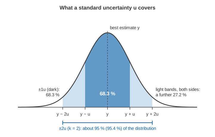
If the spread of plausible values is roughly bell-shaped (a normal distribution), the interval y ± u covers about 68 % of it, and y ± 2u about 95 %.
Combining sources: root sum of squares and sensitivity coefficients
A discharge is never measured directly. It is calculated from other quantities: width, depth, velocity, stage, a coefficient. Each has its own uncertainty, and the GUM's law of propagation of uncertainty combines them [1].
Two ideas do all the work.
1. Sensitivity coefficient. How much does the result change when one input changes a little? That ratio is the sensitivity coefficient, c. If Q = W × d × V (width × mean depth × mean velocity), then a 1 m error in width changes Q by d × V, so c for width is d × V.
2. Root sum of squares. For independent inputs, multiply each standard uncertainty by its sensitivity coefficient and add the squares, then take the square root:
u(Q) = √[ (c_W · u(W))² + (c_d · u(d))² + (c_V · u(V))² ]For a product of inputs like Q = W × d × V, this becomes even simpler in relative terms: the relative standard uncertainties combine directly [1]:
u(Q)/Q = √[ (u(W)/W)² + (u(d)/d)² + (u(V)/V)² ]If an input appears with a power, its relative uncertainty is multiplied by that power. A rating curve Q = C (h − h0)^b is the important hydrological case: a stage error Δh produces a relative discharge error of about b × Δh / (h − h0). With b = 1.8 and a 5 mm stage uncertainty, that is 1.8 × 0.005 / 0.40 = 2.3 % when the depth over the control is 0.40 m, but only 1.8 × 0.005 / 2.0 = 0.45 % at 2.0 m (illustrative values). Level matters most at low flow. The WMO Manual makes the same point through the sensitivity of a control: a 5 mm stage uncertainty gives 1 % in discharge where a 1 % change in discharge moves the stage by 5 mm, but 10 % where it moves it by only 0.5 mm [4].
Squares are used because independent errors rarely all reach their limits together in the same direction; some partly cancel.
Expanded uncertainty and the coverage factor
A standard uncertainty covers only about two-thirds of the plausible values. Users usually want a wider interval, so the GUM defines the expanded uncertainty:
U = k · u(Q)where k is the coverage factor. When the distribution is close to normal and the uncertainty is based on enough information, k = 2 gives an interval with a level of confidence of approximately 95 % [1]. The WMO Manual uses the same convention: standard uncertainties at about 68 %, expanded uncertainties at about 95 % [4]. Multiplying by k adds no new information; it only presents the same information as a wider interval [1]. That is why a reported ± is meaningless unless k is stated alongside it.
A worked example: discharge at an index-velocity station
The numbers below are illustrative. They describe a plausible mountain-river section, not a real station.
A radar measures surface velocity from a bridge and a level sensor measures stage. Mean velocity comes from surface velocity times an index coefficient (the ratio of mean to surface velocity, established at the site from gaugings). Area comes from stage and a surveyed cross-section, here summarised by mean width and mean depth:
Width W         = 40.0 m
Mean depth d    = stage − mean bed level = 1.50 m
Surface velocity = 1.50 m/s, index coefficient = 0.80
Mean velocity V = 0.80 × 1.50 = 1.20 m/s
Q = W × d × V = 40.0 × 1.50 × 1.20 = 72.0 m³/s
Step 1. Standard uncertainty of each input.
- Width, from the positions of the water's edges on the survey: u(W) = 0.20 m (Type B), or 0.20 / 40.0 = 0.5 %.
- Depth has two parts: the stage reading, u = 0.010 m (Type B, from calibration information), and the mean bed level from the survey, u = 0.030 m (Type B). Combined: √(0.010² + 0.030²) = 0.032 m, or 0.032 / 1.50 = 2.1 %.
- Velocity also has two parts. Ten surface-velocity readings had a standard deviation of 0.15 m/s, so the uncertainty of their mean is 0.15 / √10 = 0.047 m/s, or 3.2 % (Type A). The index coefficient has u = 0.032, or 4.0 % (Type B, taken from the site's calibration report). Combined: √(3.2² + 4.0²) = 5.1 %, or 0.061 m/s.
Step 2. Sensitivity coefficients. c_W = d × V = 1.80 m²/s; c_d = W × V = 48.0 m²/s; c_V = W × d = 60.0 m².
Step 3. The uncertainty budget, a table of every source and its contribution to the result.
| Source | Evaluation | Value | Standard uncertainty | Sensitivity coefficient | Contribution to u(Q) | Share of variance |
|---|---|---|---|---|---|---|
| Width W | Type B | 40.0 m | 0.20 m (0.5 %) | 1.80 m²/s | 0.36 m³/s | 0.8 % |
| Depth d (stage + bed survey) | Type B | 1.50 m | 0.032 m (2.1 %) | 48.0 m²/s | 1.52 m³/s | 14.5 % |
| Velocity V (readings + index coefficient) | Type A + Type B | 1.20 m/s | 0.061 m/s (5.1 %) | 60.0 m² | 3.67 m³/s | 84.7 % |
| Combined, u(Q) | 72.0 m³/s | 3.99 m³/s (5.5 %) | 100 % | |||
| Expanded, U (k = 2) | 8.0 m³/s (11 %) |
The arithmetic: √(0.36² + 1.52² + 3.67²) = √(0.13 + 2.30 + 13.47) = √15.9 = 3.99 m³/s. In relative terms, √(0.5² + 2.1² + 5.1²) = 5.5 %, the same answer. Doubling gives U = 8.0 m³/s.
The budget tells you where to spend effort. Halving the width uncertainty would change almost nothing; improving the index coefficient through more gaugings across the range of flows would cut the total most.
For comparison, the WMO Manual's worked current-meter gauging (20 verticals, two points per vertical, 3-minute exposures) has a combined standard uncertainty of 2.89 %, about 3 % [4]. Careful gaugings of that kind are the reference against which index coefficients and rating curves are set. The methods themselves are standardised in ISO 748:2021, which covers velocity-area gauging with point velocity devices, from current meters and acoustic Doppler instruments to floats and other surface velocity systems [2]. For how such gaugings are made, see the velocity-area method.
Try it yourself
Set the values and standard uncertainties below and watch the combined and expanded uncertainty of Q respond. Once one source dominates, the small ones hardly matter.
Illustrative calculator. It assumes the three inputs are independent and the result roughly normal; the starting values are those of the worked example.
Why a rating curve's uncertainty grows outside the gaugings
Most continuous discharge records come from a rating curve fitted to gaugings (see rating curves and their uncertainty). Inside the range of the gaugings the curve is pinned down by data; outside it, only by its fitted shape.
On log-log paper the fitted curve is a straight line. The uncertainty of its slope (the exponent b) is multiplied by the distance from the centre of the data, so it hardly matters mid-range and dominates far beyond the highest gauging; a worked example of how fast that error grows is in the rating-curve article linked above. The larger risk is physical: overbank flow or a bridge opening can change the shape of the curve at high stage, and no statistic from lower gaugings can see that. The WMO Manual states that extrapolations of rating curves are always subject to error, and recommends hydraulic reasoning or indirect peak-flow methods to reduce it [5]. Bayesian methods such as BaRatin combine prior hydraulic knowledge of the controls with the individual uncertainty of each gauging [7]. A cross-section that has changed since its survey adds another term; see river cross-section surveys.
How large can the total be? A review of observational uncertainty in hydrology found discharge uncertainty dominated by flow condition and gauging method, and easily found examples, for rainfall, discharge and water quality alike, where relative errors exceeded 40 % [6].
How to report uncertainty with water data
The GUM recommends that a reported result states the value, the expanded uncertainty with units, the coverage factor, and the approximate level of confidence, and that uncertainties are rounded to at most two significant digits [1]. For water data, a good record line looks like this:
Q = 72.0 m³/s ± 8.0 m³/s (expanded uncertainty, k = 2, about 95 %);
method: index velocity; within calibrated range: yes
Good practice for a database:
- Store uncertainty with every value, not in a separate report that gets lost.
- Flag measured, derived and extrapolated values differently. A gauging is measured, a rating-curve value is derived, and a value above the highest gauging is extrapolated.
- Keep the budget. The GUM asks for every input, its standard uncertainty, how it was obtained, and any correlations [1]. A short table like the one above is enough.
- Version the rating and cross-section that produced each value.
Common mistakes
Adding uncertainties linearly. In the worked example, adding the three contributions gives 0.36 + 1.52 + 3.67 = 5.55 m³/s instead of 3.99 m³/s, almost 40 % too high. Linear addition is correct only when the sources are fully correlated [1].
Quoting resolution as uncertainty. Resolution is the smallest step the display can show. Rounding to a 1 mm step alone contributes a standard uncertainty of 0.29 mm, which the GUM derives from a rectangular distribution [1]. That is only one component; datum errors, installation, waves, temperature and drift are usually far larger. See accuracy, resolution and precision.
Ignoring correlation. Root sum of squares assumes the inputs are independent. Two common cases break that assumption:
- Errors that do not average out. Every daily discharge in a month uses the same index coefficient, so its 4 % uncertainty pushes every day the same way and does not shrink in the monthly volume. Treating the days as independent would wrongly divide it by √30, to 0.7 %. The GUM shows the same trap with ten resistors calibrated against one standard [1].
- Errors that cancel. If stage and bed level are both referred to the same benchmark, an error in the benchmark shifts both equally and cancels in the depth.
Widening the ± instead of correcting a known bias. If a sensor reads 12 mm high, correct it; the GUM warns against enlarging the uncertainty instead [1].
Not stating k. "±8 %" could be a standard or an expanded uncertainty, a factor of two apart.
Key points
- Error is unknowable; uncertainty is the stated spread of values that could reasonably be true.
- Type A uses statistics of repeated readings, Type B everything else; both give a standard uncertainty.
- Combine independent sources by root sum of squares, weighted by sensitivity coefficients.
- Expanded uncertainty U = k × u; k = 2 gives about 95 %. Always state k.
- A budget shows which source dominates and where effort pays off.
- Rating-curve uncertainty grows beyond the gaugings, and physical changes at high flow add more.
- Report value, U, k and method together.
At ClimMaTech we keep an uncertainty budget in mind whenever we plan a monitoring station, because level and velocity feed directly into it. Tarang is our AWLR (automatic water level recorder); PRAVAAH is both an AWLR and an SVR (surface velocity radar), and gives non-contact discharge from a surveyed cross-section and a site-calibrated surface coefficient, the same ingredients as the budget above.
References
- Joint Committee for Guides in Metrology, Evaluation of measurement data: Guide to the expression of uncertainty in measurement, JCGM 100:2008 (GUM 1995 with minor corrections), BIPM, 2008. doi.org/10.59161/JCGM100-2008E
- International Organization for Standardization, Hydrometry: Measurement of liquid flow in open channels: Velocity area methods using point velocity measurements, ISO 748:2021, ISO, 2021. iso.org/standard/72754.html
- International Organization for Standardization, Hydrometric uncertainty guidance (HUG), ISO 25377:2020 (replaces ISO/TS 25377:2007), ISO, 2020. iso.org/standard/69367.html
- World Meteorological Organization, Manual on Stream Gauging, Volume I: Fieldwork, WMO-No. 1044, Chapter 10 (Uncertainty of discharge measurements) and Section 3.2 (sensitivity of controls), WMO, 2010. old.wmo.int (PDF)
- World Meteorological Organization, Manual on Stream Gauging, Volume II: Computation of Discharge, WMO-No. 1044, Sections 1.1 and 1.11 (extrapolation of rating curves), WMO, 2010. old.wmo.int (PDF)
- H. McMillan, T. Krueger, J. Freer, Benchmarking observational uncertainties for hydrology: rainfall, river discharge and water quality, Hydrological Processes 26(26), 4078–4111, 2012. doi.org/10.1002/hyp.9384
- J. Le Coz, B. Renard, L. Bonnifait, F. Branger, R. Le Boursicaud, Combining hydraulic knowledge and uncertain gaugings in the estimation of hydrometric rating curves: A Bayesian approach, Journal of Hydrology 509, 573–587, 2014. doi.org/10.1016/j.jhydrol.2013.11.016
- K. Adhikari, Y. Choden, T. Cheki, L. Gurung, T. Denka, V. Gupta, Performance evaluation of satellite precipitation estimation with ground monitoring stations over southern Himalayas in Bhutan, Acta Geophysica 68(3), 933–943, 2020. doi.org/10.1007/s11600-020-00434-z