
How to measure canal discharge: flumes, weirs and radar
The structures, gate ratings and non-contact radar methods used to measure flow in irrigation canals, with the standard equations, worked examples and a calculator.

A canal division releases water at the head regulator, and a week later the farmers at the tail say they received almost nothing. Was the water lost to seepage, taken by outlets upstream, or never released at all? Nobody can answer without numbers. Knowing how to measure discharge in a canal, meaning the volume of water passing a section each second (m³/s), is what turns that argument into water accounting. This article explains the main options: weirs and flumes, current-meter gauging, gate ratings and non-contact radar, with the standard equations and what goes wrong in the field.
Why canal discharge matters
Irrigation takes roughly 80 % of the water used in India, according to the Central Water Commission (CWC). Its 2014 guidelines give typical conveyance efficiencies of 55–60 % for unlined canals and 70–75 % for lined ones, and an overall efficiency of 30–65 % for surface-water systems [2]. In other words, much of what leaves a reservoir never reaches a crop. The same guidelines recommend charging for irrigation water on a volumetric basis and fixing outlet sizes to match crop needs [2]. Neither is possible unless flows are measured.
Measurement also matters for fairness. On a distributary of the Tungabhadra Left Bank scheme in Karnataka, a field study backed by flow measurements found that distribution followed no consistent rule. It was a series of compromises by field staff, and it explained "the widespread phenomenon of head reaches taking too much water, leaving little or nothing for the tail end" [1]. A discharge record at the head of each branch, and ideally at the tail, is the simplest check that the planned share actually arrives.
How do you measure discharge in a canal?
You measure discharge in a canal in one of three ways: with a measuring structure that has a known relation between upstream water level and discharge; by velocity-area gauging, which measures velocity across a section and multiplies it by area; or by non-contact radar, which measures water level and surface velocity from above a section of known shape. Gates and regulators can also be rated, but with more uncertainty.
A measuring structure (a weir or a flume) forces the flow through critical depth, the depth at which a given discharge passes with the least energy. Downstream conditions then cannot affect the upstream level, so a single water-level reading (the head) fixes the discharge. Such a structure is said to run under free or modular flow. When the tailwater rises too high, the structure is submerged (non-modular). The ratio of downstream to upstream head at which this begins is the modular limit [3][4]. Most of what follows concerns these discharge measurement structures, because they are the workhorses of canal measurement.
The weir method of discharge measurement
A sharp-crested or thin-plate weir is a plate with a notch, set across the channel, with an edge only 1–2 mm thick so that the water springs clear of it. The falling sheet of water is the nappe, and air must reach the space beneath it [3][4]. The head h1 is the height of the upstream water surface above the crest. It must be read where the water is not yet drawing down towards the notch: at least four times the maximum head upstream of the weir, according to the US Bureau of Reclamation (USBR) Water Measurement Manual [3].
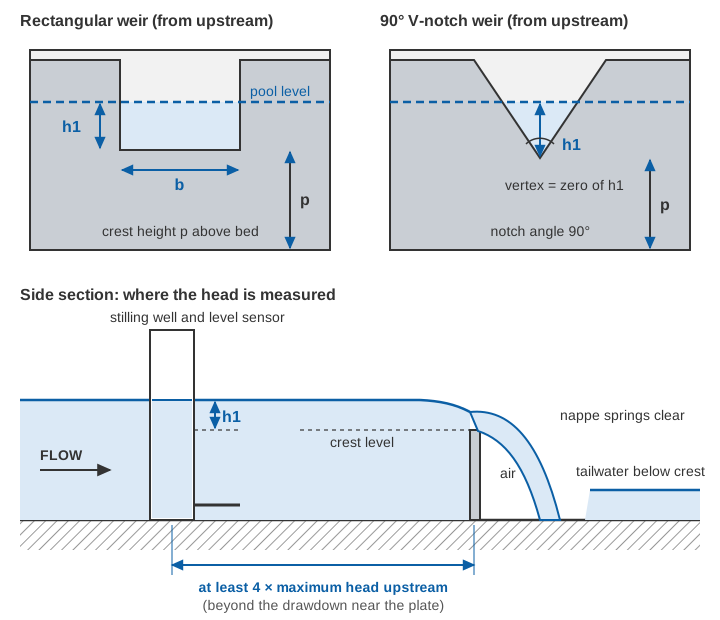
Thin-plate weirs are standardised internationally in ISO 1438, adopted in India as IS 9108:2020, Hydrometry: open channel flow measurement using thin-plate weirs [5]. The equations below are the Kindsvater–Carter forms given in the USBR manual and in the Bos handbook [3][4].
What is the weir discharge formula?
For a rectangular weir, the weir discharge formula is the Kindsvater–Carter equation, which adds small corrections to the measured width and head:
Rectangular weir:   Q = Ce × (2/3) × √(2g) × be × he^1.5

be = b + kb     (effective crest width, m)
he = h1 + kh    (effective head, m; kh = 0.001 m)
Ce = effective discharge coefficient, a function of b/B and h1/p
     for a full-width weir (b = B):  Ce = 0.602 + 0.075 × h1/p
B  = width of the approach channel, p = crest height above the bed
Values of kb and Ce for other width ratios come from published curves and tables [3][4]. For a full-width weir kb is about −0.9 mm (−0.003 ft on the USBR curve) [3].
For a triangular notch (V-notch), the Kindsvater–Shen equation is:
V-notch weir:   Q = Ce × (8/15) × √(2g) × tan(θ/2) × he^2.5

he = h1 + kh,   θ = notch angle
fully contracted 90° notch:  Ce ≈ 0.578,  kh ≈ 0.0029 ft ≈ 0.9 mm
The 90° values are read from the USBR curves of Ce and kh against notch angle [3]. Because discharge rises with the 2.5 power of head, a V-notch spreads small flows over a usable range of head. That is why it is the usual choice for small canals, outlets and seepage measurement.
Bos recommends a minimum head of 0.03 m on a rectangular weir, h1/p no greater than 2.0, a crest height of at least 0.10 m and a crest width of at least 0.15 m. For a fully contracted V-notch, the head should stay between 0.05 and 0.38 m [4]. With reasonable care in construction, the error in Ce is expected to be under about 1 % [4].
The cost of this accuracy is head loss. Because the nappe must stay ventilated, the water level downstream has to sit below the crest, so a sharp-crested weir needs a total drop of more than its own head plus about 0.05 m [4]. The weir also creates a pool in which silt settles, and the USBR manual requires the approach to be kept free of sediment deposits [3]. On flat command areas carrying silty water, both are serious drawbacks. And once the tailwater rises above the crest, USBR states plainly that accurate measurement "should not be expected" [3].
Broad-crested weirs and standing wave flumes
A broad-crested weir has a flat crest long enough for the streamlines over it to be nearly parallel. Its ideal equation is Q = (2/3) × √(2g/3) × b × H1^1.5, with H1 the upstream energy head above the crest. In practice it is multiplied by a discharge coefficient and a velocity-of-approach correction [4]. The rectangular broad-crested weir is covered by IS 14974:2018, identical to ISO 3846:2008 [7]. Broad-crested weirs and long-throated flumes tolerate much higher tailwater than thin plates. USBR gives modular limits of 72–93 % for long-throated flumes without an expansion section [3].
Indian canals also use standing wave flumes, standardised in IS 6063:1971 and, with a fall downstream, in IS 6062:1971 [8][9]. Their foreword notes two practical merits: only one upstream gauge reading is needed, and the modular relationship stays constant "even with the sediment deposition in the upstream side" [8].
How does a Parshall flume work?
A Parshall flume works by squeezing the flow through a narrow throat with a sloping floor, so that it passes through critical depth near the end of a level converging section. One upstream head then fixes the discharge. The flume has three parts: a converging section with a level floor, a short throat whose floor slopes down, and a diverging section whose floor rises again [4][6]. The flume is named after R. Parshall, who developed it in 1922, and it is calibrated empirically. Its sizes are not scale models of one another, so each size must be built exactly to its published dimensions [3][4].
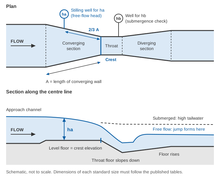
The head ha is measured on the converging wall at two-thirds of the wall length upstream of the crest, through a pipe to a stilling well, and the gauge zero is set to the crest (the level floor), not to the pipe [4][6]. In India the device is standardised in IS 14371:1996, Measurement of liquid flow in open channels: Parshall and SANIIRI flumes, which follows ISO 9826 [6].
What is the Parshall flume formula?
The Parshall flume formula is a power law in the upstream head:
Free flow:   Q = C × ha^n          (Q in m³/s, ha in m)

IS 14371 standard flumes (throat width b = 0.25 to 2.4 m):
   n = 1.569 × b^0.026
   C = 0.372 × b × 3.279^n
   e.g. b = 0.30 m:  C = 0.679, n = 1.521
        b = 0.60 m:  C = 1.403, n = 1.548
        b = 1.00 m:  C = 2.397, n = 1.569
The coefficients are those tabulated in IS 14371, and the general expression reproduces them [6]. USBR's Table 8-6 gives the same family in feet for sizes from 1 inch to 50 feet [3].
Free versus submerged flow. The flume runs free until the submergence ratio hb/ha reaches its modular limit. USBR gives 50 % for 1–3 inch flumes, 60 % for 6 and 9 inch, 70 % for 1–8 ft and 80 % for 8–50 ft [3]. IS 14371 quotes experimental modular limits of 0.55 to 0.78 across its standard sizes [6]. Above the limit, a correction read from charts is subtracted from the free-flow discharge. Above 95 % submergence the flume no longer measures at all [6]. Correcting for submergence costs accuracy: USBR estimates that head-reading imprecision adds 4 to 20 % to the free-flow accuracy of 3 to 5 % [3].
Accuracy and limits. IS 14371 gives a systematic uncertainty of 2 to 4 % in the Parshall coefficient. Its worked example, a 1.0 m flume at 0.6 m head, gives 1.075 m³/s ± 3.8 % [6]. Head loss through a flume is less than about a quarter of that needed by a sharp-crested weir of the same control width [3]. The flume's approach must still be kept clean, because changing downstream resistance from silt, weeds or canal checking can push a free-flowing flume into submergence [3][6]. For new installations, the USBR manual now also describes long-throated flumes, which can be rated by computation and designed for higher submergence limits, and states that "long-throated flumes are preferred over Parshall flumes for new installations". It keeps the Parshall dimensions and tables "because so many Parshall flumes are currently in use", mainly for checking existing flumes [3].
Worked examples
A 90° V-notch at 0.20 m head (illustrative)
he  = 0.200 + 0.0009            = 0.2009 m
he^2.5 = 0.2009² × √0.2009 = 0.04036 × 0.4482 = 0.018091
Ce × (8/15) × √(2 × 9.81) × tan 45° = 0.578 × 0.5333 × 4.429 × 1 = 1.3655
Q   = 1.3655 × 0.018091          = 0.02470 m³/s ≈ 24.7 L/s
The rating table for 90° notches in Bos, adapted from ISO tables, lists 24.72 L/s at 0.200 m [4]. Now suppose the gauge zero is 2 mm out. At 0.198 m and 0.202 m the same equation gives 24.1 and 25.3 L/s, about ±2.5 % for ±2 mm. With a 2.5 power, every 1 % error in head becomes about 2.5 % in discharge. That is why setting the zero matters as much as the coefficient.
A 0.60 m Parshall flume at 0.45 m head (illustrative)
n  = 1.569 × 0.60^0.026       = 1.548
C  = 1.403                    (IS 14371, b = 0.60 m)
Q  = 1.403 × 0.45^1.548 = 1.403 × 0.2905 = 0.408 m³/s
Check submergence. If the throat well reads hb = 0.29 m, then hb/ha = 0.29 / 0.45 = 0.64. That is below the 70 % limit USBR gives for flumes of this size [3], so the flow is free and the reading stands. If hb were 0.36 m (80 %), the flume would be submerged and a correction from IS 14371 would be needed [6]. A 3 mm zero error on ha changes Q by about 1.548 × 3/450 ≈ 1.0 %.
Try it yourself
Current meters, gate ratings and the float method
Where no structure exists, discharge is measured by the velocity-area method. A current meter reads velocity at set depths on a series of verticals, and the panel discharges are summed. It is the reference method for checking structures and calibrating everything else. We describe it step by step in the velocity-area method. In a lined canal the section is regular and easy to gauge, but each gauging is a single visit, not a record. Floats give a rough surface velocity when nothing else is available.
Head regulators and cross regulators can also serve as meters. For flow under a vertical gate, Bos gives:
Q = Ce × b × w × √(2g × y1)

b = gate width, w = gate opening, y1 = upstream depth
Ce depends on y1/w and, under submerged flow, on the tailwater depth
Under free flow the laboratory coefficients are well defined. Bos warns of "considerable errors" in submerged flow when upstream and downstream depths are close [4]. In the field, gate seals, sills and openings rarely match laboratory conditions, so a gate rating should be checked against current-meter gaugings. A regulator rating is a rating curve like any other, with the same need for periodic checks; see rating curves and their uncertainty. For orifice flow under spillway gates, see how dam spillways and gates work.
Non-contact radar at a lined canal section
A structure costs head and space, and many existing canals have neither to spare. The alternative is to measure area and velocity directly at a section whose shape is known:
- A level radar above the water measures the distance down to the surface, which gives the water level. With a surveyed cross-section, the level gives the flow area
A. - A surface velocity radar (SVR) aimed at an angle along the canal measures the Doppler shift of radar echoes from the surface. The echo comes from Bragg scattering, reflection from short ripples whose spacing matches the radar wavelength [11]. The radar therefore needs a moving, rippled surface.
- A coefficient
kconverts surface velocity to mean velocity:Q = A × k × v_surface.
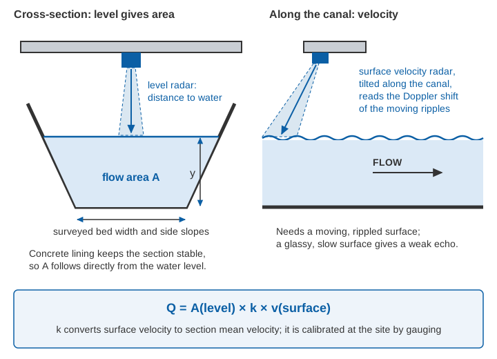
Lined canals suit this well. Concrete lining keeps the cross-section from changing, so the area follows directly from the level. The flow is usually fast enough to keep the surface rippled. There is nothing in the water to silt up, and no head is lost. Mounting height, beam clearance, tilt and setting the zero are covered in how to install radar level and velocity sensors on a bridge.
The coefficient is the weak point. In tests on the San Joaquin and Cowlitz rivers, mean velocity was about 0.85 times surface velocity [11]. Field trials of a portable SVR at several sites confirmed 0.85 as a reasonable default, but recommended site-specific calibration. In very smooth channels the default underestimates discharge, and in very rough ones it overestimates [10]. A concrete-lined canal is at the smooth end, so the true k is likely to be higher than 0.85. It must be measured with current-meter gaugings at the site over the range of operating levels.
Illustrative example. Take a lined trapezoidal canal with a bed width of 3.0 m, side slopes of 1.5 horizontal to 1 vertical, a depth of 1.20 m and a surface velocity of 1.10 m/s:
A = (3.0 + 1.5 × 1.20) × 1.20 = 4.80 × 1.20 = 5.76 m²
k = 0.85:  Q = 5.76 × 0.85 × 1.10 = 5.39 m³/s
k = 0.90:  Q = 5.76 × 0.90 × 1.10 = 5.70 m³/s   (+5.9 %)
A 0.05 change in k moves the answer by about 6 %, more than the whole uncertainty of a good flume. With a calibrated coefficient, fixed radar stations have tracked conventional streamgauge records closely in long trials [11][12]. The physics of the velocity radar is explained in surface velocity radar: how Doppler measures river flow, and the wider question in can radar measure river discharge?.
Comparing the methods
| Method | Typical accuracy (source) | Head loss | Silt and debris | Effort | Continuous record |
|---|---|---|---|---|---|
| Thin-plate weir (rectangular, V-notch) | Coefficient within about 1 % with careful construction [4] | High: drop greater than the head plus about 0.05 m [4] | Poor: pool silts up; approach must be kept clear [3] | Simple plate, but needs a drop and a clean pool | Yes, with a level sensor in a stilling well |
| Broad-crested weir, long-throated flume | Long-throated flumes about 2–5 %, depending on head measurement [3] | Low; modular limits of 72–93 % [3] | Better: flat floors pass sediment [3][4] | Civil works to standard shape | Yes, one upstream head |
| Parshall flume | Free flow 3–5 % [3]; coefficient 2–4 % [6] | Under a quarter of a weir's [3]; modular limit 50–80 % [3] | Fair; downstream silt can submerge it [3] | Exact construction to the size's dimensions [3] | Yes; two heads if submerged |
| Gate or regulator rating | Free-flow coefficients about 2 % in the laboratory [4]; worse when submerged | None beyond the gate's own | Sills and seals change with silt | Needs gauging to check | Yes, with gate opening and levels |
| Current meter (velocity-area) | Reference method; see the velocity-area method | None | Unaffected | A field team for every gauging | No, one visit at a time |
| Level radar + SVR | Within 10 % in field trials with a theoretical or site-calibrated coefficient, for low to intermediate roughness [10] | None | Unaffected; nothing in the water | Section survey and calibration gaugings | Yes |
The accuracies come from sources that define them differently, so treat them as orders of magnitude. Every installation adds the uncertainty of its level measurement, construction and maintenance.
Choosing for your canal
A few practical rules follow from the standards:
- Small flows, enough drop, clean water: a V-notch or rectangular thin-plate weir is cheap and accurate.
- Silty canals with little drop: a long-throated flume, broad-crested weir or standing wave flume. The Parshall flume is common, but only when built exactly to its dimensions and kept below its modular limit.
- An existing lined section where nothing can be built: level radar with SVR, calibrated by gaugings.
- Always: set the gauge zero carefully, check it after every maintenance season, and confirm the rating with an independent gauging from time to time. A structure that is silted, submerged or out of level gives a confident wrong number. Datum checks are covered in gauge zero, datum and benchmarks.
Key points
- Canal discharge measurement underpins water accounting, volumetric charging and a fair share for tail-end farmers.
- Weirs and flumes give discharge from one head reading, provided they run free and the head is measured at the specified point.
- Thin-plate weirs are the most accurate but need a drop and a clean pool. Flumes and broad-crested weirs lose less head and tolerate silt better.
- The Parshall flume formula is
Q = C·ha^n, withhameasured at two-thirds of the converging wall upstream of the crest. Above the modular limit it needs a correction. - Gate ratings and radar both need checking against current-meter gaugings. For radar, the surface-to-mean velocity coefficient is the key calibration.
Where ClimMaTech fits
At ClimMaTech we work on canal monitoring where a new structure is not an option. PRAVAAH is a non-contact discharge sensor that combines an AWLR (Automatic Water Level Recorder) with an SVR (Surface Velocity Radar). With a surveyed cross-section and a site-calibrated coefficient, it reports discharge at a canal section. Our canal irrigation monitoring page describes how level and velocity readings at regulators, branches and tail reaches fit together.
References
- M. Jurriëns, M. Kuper, Water distribution on a large distributary, Tungabhadra, India: design and formal operation vs. actual procedures, Irrigation and Drainage Systems 9(1), 85–103, 1995. doi:10.1007/BF00881590
- Central Water Commission, Ministry of Water Resources, Guidelines for Improving Water Use Efficiency in Irrigation, Domestic & Industrial Sectors, November 2014. cwc.gov.in
- U.S. Bureau of Reclamation, Water Measurement Manual, 3rd edition, revised reprint, 2001, chapters 7 (weirs) and 8 (flumes). usbr.gov
- M. G. Bos (editor), Discharge Measurement Structures, Publication 20, 1st edition, International Institute for Land Reclamation and Improvement (ILRI), Wageningen, 1976. edepot.wur.nl
- Bureau of Indian Standards, IS 9108:2020 / ISO 1438:2017, Hydrometry: open channel flow measurement using thin-plate weirs (second revision). services.bis.gov.in
- Bureau of Indian Standards, IS 14371:1996, Measurement of liquid flow in open channels: Parshall and SANIIRI flumes (ISO 9826), reaffirmed 2003. archive.org (Public.Resource.Org) (archived copy)
- Bureau of Indian Standards, IS 14974:2018 / ISO 3846:2008, Hydrometry: open channel flow measurement using rectangular broad crested weirs (first revision). services.bis.gov.in
- Bureau of Indian Standards, IS 6062:1971, Method of measurement of flow of water in open channels using standing wave flume-fall. services.bis.gov.in
- Bureau of Indian Standards, IS 6063:1971, Method of measurement of flow of water in open channels using standing wave flume. services.bis.gov.in
- M. Welber, J. Le Coz, J. B. Laronne, G. Zolezzi, D. Zamler, G. Dramais, A. Hauet, M. Salvaro, Field assessment of noncontact stream gauging using portable surface velocity radars (SVR), Water Resources Research 52(2), 1108–1126, 2016. doi:10.1002/2015WR017906
- J. E. Costa, R. T. Cheng, F. P. Haeni, N. Melcher, K. R. Spicer, E. Hayes, W. Plant, K. Hayes, C. Teague, D. Barrick, Use of radars to monitor stream discharge by noncontact methods, Water Resources Research 42(7), 2006. doi:10.1029/2005WR004430
- J. W. Fulton, C. A. Mason, J. R. Eggleston, M. J. Nicotra, C.-L. Chiu, M. F. Henneberg, H. R. Best, J. R. Cederberg, S. R. Holnbeck, R. R. Lotspeich, C. D. Laveau, T. Moramarco, M. E. Jones, J. J. Gourley, D. Wasielewski, Near-field remote sensing of surface velocity and river discharge using radars and the probability concept at 10 U.S. Geological Survey streamgages, Remote Sensing 12(8), 1296, 2020. doi:10.3390/rs12081296