
Weather radar vs rain gauge vs satellite: who sees what
How each of the three measures rain, what a dBZ number means, where each one goes wrong in the mountains, and which to rely on when a flood warning is at stake.

Imagine heavy rain over a hill district. The rain gauge at the block office shows 38 mm in the last hour. The IMD radar image shows a band of orange and red echoes a little to the north. A satellite map the next morning shows a moderate total spread over the whole area. The three do not agree. This is the everyday reality of weather radar vs rain gauge vs satellite: each sees a different part of the same storm, at a different scale and with a different delay. Knowing who sees what tells you which number to trust for a flood warning.
Weather radar vs rain gauge: a point against an area
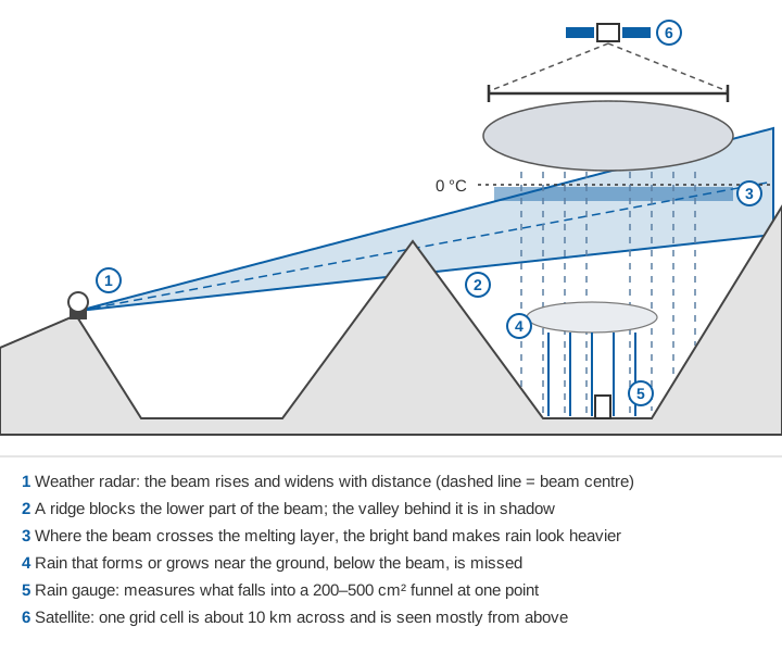
A rain gauge measures what falls into its funnel. WMO's Guide to Hydrological Practices notes that a collector of 200 to 500 cm² is the most convenient size [1]. The gauge is the most direct measurement we have, but it describes one point. It also reads low, because wind carries drops around the opening and some water is lost to evaporation, splashing and wetting. The undercatch is about 5 % in heavy rain and larger in drizzle, snow and wind [2]. Gauge density, gauge types and India's networks are covered in how many rain gauges does a district need, types of rain gauges used in India and India's automatic weather station and rain gauge networks.
A weather radar measures an average over a volume of air. At 160 km from the radar the beam may be several kilometres wide. WMO therefore warns that radar rainfall should not be expected to correlate highly with a single gauge. But the areal pattern a radar shows is usually much more representative of the storm than most gauge networks [1].
Worked example: how big is each footprint?
The numbers below are illustrative, for a site near 31°N in the western Himalaya. One degree of latitude is about 111.3 km; one degree of longitude is 111.3 km × cos(latitude).
| Sensor | Footprint | Area |
|---|---|---|
| Rain gauge, 200 cm² funnel | one point | 0.00000002 km² |
| Radar range bin, 1 km long × 1° wide, at 100 km | 1 km × (100 km × 0.01745) | about 1.7 km² |
| CHIRPS grid cell, 0.05° | 5.57 km × 4.77 km | about 27 km² |
| IMERG grid cell, 0.1° | 11.13 km × 9.54 km | about 106 km² |
One IMERG cell is about five billion times the area of a gauge funnel. When a gauge and a satellite cell disagree, both may be right about what they measured.
How does Doppler weather radar work?
A Doppler weather radar sends out a very short pulse of microwaves, listens for the echo from raindrops, snow or hail, and times it to find the distance. In the US network, each pulse lasts 1.57 millionths of a second and is repeated about 1,300 times a second [3]. Scanning at a series of elevation angles, it completes a full volume in a few minutes [1][3].
The strength of the echo depends on the radar reflectivity factor, Z. For raindrops, which are small compared with the wavelength, the echo is proportional to the sixth power of drop diameter, summed over the drops in the beam [1]. That sixth power matters: one 4 mm drop returns as much power as 4,096 drops of 1 mm.
Weather radars use S-band (about 10 cm), C-band (about 5–6 cm) and X-band (about 3 cm) [1]. The longer the wavelength, the less the rain itself weakens the beam; shorter wavelengths detect light rain and snow more readily.
What "Doppler" adds
When the pulse hits a moving target, the phase of the returned wave shifts. The radar uses that shift to work out how fast the target is moving towards or away from it [3]. Only this radial component, along the beam, is measured. For a target moving with radial speed v, the Doppler frequency shift is:
f_D = 2 v / λ
Example: v = 10 m/s, λ = 5 cm (C-band)
f_D = 2 × 10 / 0.05 = 400 Hz
Doppler data are used to estimate winds, to give early signs of tornadoes and severe storms, and to filter out ground clutter, which does not move [1]. In India, IMD uses its Doppler weather radars (DWRs) mainly to monitor localised thunderstorms and heavy rainfall and to issue nowcast warnings for up to 3 hours. The data are also fed into nowcast models that predict rainfall and thunderstorms 6 to 12 hours ahead [4].
Dual polarisation, briefly
A dual-polarised radar receives echoes in both horizontal and vertical planes [5]. Differential reflectivity (ZDR), the power difference between them, tells flattened raindrops from round, tumbling hail. The correlation coefficient falls in mixed rain and snow, hail, and non-weather echoes such as birds and smoke. Specific differential phase (KDP) shows how much the rain slows the beam and improves rainfall estimates [5].
What is weather radar dBZ?
dBZ is radar reflectivity expressed in decibels, a logarithmic power ratio relative to the reflectivity factor Z [6], with Z in mm⁶/m³:
dBZ = 10 × log10( Z / 1 mm⁶ m⁻³ )
Z = 200 R^1.6        (rain; R in mm/h)
so  R = ( 10^(dBZ/10) / 200 )^(1/1.6)
Example: 40 dBZ → Z = 10,000 → R = (10,000 / 200)^0.625 = 11.5 mm/h
Precipitation gives values from about 0 dBZ in very light rain to more than 60 dBZ in extremely heavy rain or hail [6]. The link to rain rate is an empirical Z–R relation, and WMO describes Z = 200 R^1.6 as the most common one in use [1]. Under it, 30 dBZ is about 3 mm/h, 40 dBZ about 12 mm/h, 50 dBZ about 47 mm/h and 60 dBZ about 205 mm/h [7].
No single Z–R relation fits all rain, because drop sizes differ from storm to storm. For snow, WMO quotes typical values of Z = 2000 R^2.0 [1]. In a strong downdraft of 8 m/s, reflectivity for a given rain rate is about 3 dB lower than in still air, and rain is underestimated by about 40 % [1]. Try it below.
Illustrative: the relations are typical values quoted by WMO [1]; operational radars may use locally fitted relations.
Notice what a small calibration error does. With b = 1.6, a 1 dB error changes the rain rate by a factor of 10^(1/16) ≈ 1.15, or 15 %. A 2 dB error changes it by about 33 %. That is why gauges are used to check radar rainfall.
How many Doppler weather radars does India have?
In a written reply to Parliament on 12 December 2024, the government stated that 39 Doppler weather radars were installed across the country [4]. They were a mix of S-band, C-band and X-band. The Himalayan sites on that list are all X-band: Kufri, Jot and Murari Devi in Himachal Pradesh; Mukteshwar, Surkanda Devi and Lansdowne in Uttarakhand; Srinagar, Jammu and Banihal Top in Jammu & Kashmir; and a transportable radar at Leh [4]. Mission Mausam, launched in September 2024, planned 87 more by 2026 [4].
On 2 April 2025 the government listed the planned sites, including an X-band radar for Lahaul & Spiti, plus 53 further radars across the country [8]. On 27 November 2025 two dual-polarised C-band radars were inaugurated at Raipur and Mangaluru. On that occasion the Secretary of the Ministry of Earth Sciences said IMD had achieved over 50 % radar coverage and was planning phased-array radars for Jammu & Kashmir, Uttarakhand and Himachal Pradesh [9]. These counts change quickly; each is as stated on its date.
Why radar struggles in the mountains
The beam rises with distance
The Earth curves away beneath the beam. Normal refraction bends the beam slightly, which is allowed for by treating the Earth as having four-thirds of its real radius [1]. The beam also spreads with distance [10]: a beam 1° wide is about 100 km × 0.01745 = 1.75 km across at 100 km.
h ≈ r × sin(θ) + r² / (2 × k × a)
a = 6,371 km (Earth radius), k = 4/3, so k × a ≈ 8,495 km
Example: r = 100 km, θ = 0.5°
h ≈ 100 × 0.00873 + 100² / 16,990 = 0.87 + 0.59 = 1.46 km above the antennaAt 150 km even the bottom of the beam is more than 1 km above the antenna, so a shallow storm in a valley can pass beneath it. WMO notes that low-level orographic growth of rain on hills facing moist winds may happen below the beam, and must then be estimated with correction factors [1].
Hills block the beam
Ridges intercept the beam, causing permanent ground clutter and screening the rain behind them. WMO says a blocked beam can be corrected only if at least 40 % of it is unobstructed [1]. In deep valleys the lowest elevation angles may be blocked in many directions.
The bright band
Melting snowflakes are still large but now wet on the outside, and they return strong echoes. Reflectivity is therefore enhanced in a layer a few hundred metres below the freezing level: the bright band [1]. Where the beam passes through it, rainfall is overestimated; above it, in snow, rainfall is underestimated. Correcting for the vertical profile of reflectivity is, in WMO's words, "an essential first step" after removing ground clutter [1]. This matters for winter precipitation in the Himalaya, much of which falls as snow, as described in western disturbances and winter precipitation.
Heavy rain weakens the beam
Rain absorbs and scatters microwaves, and the effect grows rapidly at shorter wavelengths. In WMO's table, rain of 50 mm/h attenuates a 10 cm (S-band) beam by 0.015 dB per km, a 5.7 cm (C-band) beam by 0.215 dB/km and a 3.2 cm (X-band) beam by 1.25 dB/km. An X-band beam loses 10 dB after only 8 km in such rain [1]. Corrections exist but can be unstable in severe attenuation [1].
How accurate is radar rainfall?
With careful correction, a single-polarisation radar can measure daily rainfall to within about 10 %, similar to gauges. Hourly rainfall over a catchment of about 100 km² is measured to a mean accuracy of about 20 % in widespread stratiform rain, but only about 40 % in heavy convective rain [1].
How do satellites measure rainfall?
Satellites look down from above, mostly at cloud tops, so most of their rainfall estimates are indirect [1].
- Infrared sensors on geostationary satellites measure cloud-top temperature about every 30 minutes [2]. Cold, spreading cloud tops suggest heavy rain, but rain from warmer clouds is missed [1].
- Passive microwave radiometers on low-orbiting satellites measure natural microwave emission. Over the sea, emission from raindrops can be measured; over land, rain is detected mainly through scattering by ice high in the cloud. Rain from clouds with little ice largely goes undetected [1].
- Spaceborne radar gives the most direct view. The GPM Core Observatory carries a dual-frequency precipitation radar and a microwave imager with high-frequency channels for light rain and snow. It flies in an orbit inclined at 65°, which covers more of the globe than its predecessor, TRMM [2].
IMERG
NASA's Integrated Multi-satellitE Retrievals for GPM (IMERG) combines all available microwave estimates, calibrated against the combined radar–radiometer product from the GPM core satellite. It fills the gaps between overpasses using infrared data and motion vectors [2]. Its grid is 0.1° and its time step is 30 minutes. It is produced three times: an Early run about 4 hours after observation, a Late run about 12 to 14 hours after, and a Final run about 3.5 months after the month ends [2]. Only the Final run is adjusted to monthly rain-gauge analyses from the Global Precipitation Climatology Centre; Early and Late use climatological calibration [2].
CHIRPS
The Climate Hazards group Infrared Precipitation with Stations (CHIRPS) dataset was developed to support the Famine Early Warning Systems Network, which monitors drought and food security. It covers 50°S to 50°N at 0.05° from 1981 onwards, with daily, five-day and monthly totals [11]. It estimates rain from the time cloud tops stay colder than 235 K, scaled by a high-resolution rainfall climatology, and blends in station data. A preliminary version is available after about 2 days and the final version after about 3 weeks [11]. Its strength is a long, consistent record; it is not built for hourly flood work.
Satellite rainfall data in the Himalaya: known biases
Over Indian mountains, peer-reviewed comparisons with gauges show consistent patterns:
- Against IMD gauges across the Himalayan region, the TRMM 3B42V7 product overestimated rainfall below about 3,100 m and underestimated it above. Correlation for individual rain events was only about 0.23, rising to about 0.67 for area-averaged rain, and the product was judged unsuitable for very heavy rainfall [12].
- A global comparison found large negative biases on the windward slopes of monsoon mountains in June–August. It linked them to microwave algorithms underestimating shallow orographic rain, and to sparse gauges for bias correction [13].
- Across 86 Indian basins, IMERG reduced the dependence of errors on climate and especially topography compared with TRMM [14].
- In our study of extremes across India (2007–2016), CHIRPS, SM2RAIN-ASCAT and TRMM all varied strongly from region to region in capturing extremes against IMD gridded data; TRMM and CHIRPS did best [15].
- At 32 gauges in the southern Himalaya of Bhutan (1998–2017), we found that TRMM monthly rainfall tracked the gauges (average correlation 0.81) but underestimated it, with relative error above 50 % at 96 % of stations [16].
For flood work this matters: over Indian basins, real-time satellite products were biased, sometimes high and sometimes low depending on the product, and the bias carried into simulated flood peak timing and magnitude [17].
Merged products: gauges and satellites together
Gauges are accurate but sparse; satellites cover everything but with bias; so the two are often merged. IMD's gridded daily rainfall at 0.25° was built from 6,955 quality-controlled gauges for 1901–2010 and shows orographic rainfall better than coarser datasets [18]. An early Indian merge combined TRMM satellite estimates with IMD gauges at 1° resolution, using the satellite as a first guess and the gauges to correct its mean bias [19]. IMERG Final is itself a satellite–gauge merge at the monthly scale [2]. Where gauges are few, as in much of the high Himalaya, a merge falls back on the satellite.
Comparison: who sees what
| Rain gauge | Weather radar | IMERG | CHIRPS | |
|---|---|---|---|---|
| What it measures | Water in a 200–500 cm² funnel [1] | Echo from a volume of air, converted with a Z–R relation [1] | Microwave and infrared, merged [2] | Cold-cloud duration plus stations [11] |
| Spatial scale | One point | Range bins widen with distance; the beam is several km wide at 160 km [1] | 0.1° (about 10 km) [2] | 0.05° (about 5 km) [11] |
| Time step | Minutes (automatic) to daily (manual) | A volume every few minutes [1][3] | 30 min [2] | Daily, 5-day, monthly [11] |
| Delay | As fast as its telemetry | Minutes | About 4 h (Early) to 3.5 months (Final) [2] | About 2 days to 3 weeks [11] |
| Strengths | Direct, long records, reference for others | Storm structure and motion, nowcasting, wind | Global, near real time | Long record from 1981, consistent |
| Weaknesses | One point, undercatch in wind and snow [2] | Beam height, blockage, bright band, attenuation, calibration [1] | Indirect; orographic and warm rain biases [12][13] | Too coarse in time for flash floods |
Which should you use for flood warning?
It depends on how fast your river responds. For small, steep catchments that peak within an hour or two of heavy rain, as discussed in time of concentration and flash floods vs river floods, the warning has to come from gauges inside the catchment and, where coverage allows, from radar. An IMERG Early estimate arriving about 4 hours later [2] comes after such a flood.
For large basins with long travel times, satellite rainfall is valuable over upstream areas with few or no gauges, including across borders, once its local bias has been checked against your gauges. Radar is widely used as an informal first alert, but WMO noted that only two or three countries used radar rainfall quantitatively in flow forecasting, always alongside gauges [1].
In practice the three work best together:
- Treat gauges as the reference, and keep them well sited and maintained (see tipping-bucket rain gauge errors).
- Use radar for where the storm is and where it is going in the next hours, and check its rain rates against gauges.
- Before trusting a satellite product for your catchment, compare it with local gauges over several seasons, especially above about 3,000 m.
For the full warning chain, see how a flood early warning system works.
Key points
- A gauge measures a point, radar a volume of air, a satellite a grid cell seen from above. Disagreement is expected.
- dBZ is reflectivity on a logarithmic scale. Under Z = 200 R^1.6, 40 dBZ is about 12 mm/h, and a 1 dB calibration error changes rain rate by about 15 %.
- Doppler adds radial velocity; dual polarisation helps tell rain from hail and non-weather echoes.
- In mountains, radar loses rain to beam height and blockage, is distorted by the bright band, and at X-band is weakened by heavy rain.
- IMERG (0.1°, 30 min) arrives about 4 hours after observation at the earliest; CHIRPS (0.05°, daily) after about 2 days. Satellite estimates carry known biases over Himalayan terrain.
- For flash-flood warning, gauges in the catchment come first and radar second; satellites help most for large, poorly gauged basins.
Where ClimMaTech fits
At ClimMaTech we work on ground-based rainfall and river monitoring in Himalayan catchments, where a well-sited gauge remains the reference that radar and satellite estimates are checked against. Our weather station, VARSHAQ, is in development. You can read more about how we approach warnings on the flood warning page.
References
- World Meteorological Organization, Guide to Hydrological Practices, Volume I: Hydrology – From Measurement to Hydrological Information (WMO-No. 168), 2008 edition, updated in 2020, Chapter 3 (sections 3.3, 3.7–3.9 and 3.11), WMO, Geneva. old.wmo.int (PDF)
- G. J. Huffman, D. T. Bolvin, R. Joyce, E. J. Nelkin, J. Tan, D. Braithwaite, K. Hsu, O. A. Kelley, P. Nguyen, S. Sorooshian, D. C. Watters, B. J. West, P. Xie, Algorithm Theoretical Basis Document (ATBD): NASA Global Precipitation Measurement (GPM) Integrated Multi-satellitE Retrievals for GPM (IMERG), Version 07, NASA Goddard Space Flight Center, 12 July 2023. gpm.nasa.gov
- NOAA National Weather Service JetStream, How radar works, last updated 27 September 2023. noaa.gov
- Press Information Bureau, Ministry of Earth Sciences, Parliament question: Doppler radar station at Balasore, 12 December 2024. pib.gov.in
- NOAA National Weather Service JetStream, Dual polarization, last updated 27 September 2023. noaa.gov
- NOAA National Weather Service, Glossary: dBZ, and NWS Training Center, Equivalent reflectivity (Ze). forecast.weather.gov; training.weather.gov
- NOAA National Weather Service JetStream, Radar images: Reflectivity, last updated 11 March 2025. noaa.gov
- Press Information Bureau, Ministry of Earth Sciences, Parliament question: Installation of new radar system, 2 April 2025. pib.gov.in
- Press Information Bureau, Ministry of Earth Sciences, Dr. Jitendra Singh inaugurates 3 major initiatives of IMD, two new C-band Doppler weather radars, solar panel system and meteorological museum, 27 November 2025. pib.gov.in
- NOAA National Weather Service JetStream, Radar beams, last updated 10 August 2023. noaa.gov
- C. Funk, P. Peterson, M. Landsfeld, D. Pedreros, J. Verdin, S. Shukla, G. Husak, J. Rowland, L. Harrison, A. Hoell, J. Michaelsen, The climate hazards infrared precipitation with stations — a new environmental record for monitoring extremes, Scientific Data 2, 150066, 2015. doi:10.1038/sdata.2015.66
- V. Bharti, C. Singh, Evaluation of error in TRMM 3B42V7 precipitation estimates over the Himalayan region, Journal of Geophysical Research: Atmospheres 120, 12458–12473, 2015. doi:10.1002/2015JD023779
- Z. Liu, Evaluation of precipitation climatology derived from TRMM Multi-Satellite Precipitation Analysis (TMPA) monthly product over land with two gauge-based products, Climate 3(4), 964–982, 2015. doi:10.3390/cli3040964
- H. Beria, T. Nanda, D. S. Bisht, C. Chatterjee, Does the GPM mission improve the systematic error component in satellite rainfall estimates over TRMM? An evaluation at a pan-India scale, Hydrology and Earth System Sciences 21, 6117–6134, 2017. doi:10.5194/hess-21-6117-2017
- V. Gupta, M. K. Jain, P. K. Singh, V. Singh, An assessment of global satellite-based precipitation datasets in capturing precipitation extremes: A comparison with observed precipitation dataset in India, International Journal of Climatology 40(8), 3667–3688, 2020. doi:10.1002/joc.6419
- K. Adhikari, Y. Choden, T. Cheki, L. Gurung, T. Denka, V. Gupta, Performance evaluation of satellite precipitation estimation with ground monitoring stations over southern Himalayas in Bhutan, Acta Geophysica 68(3), 933–943, 2020. doi:10.1007/s11600-020-00434-z
- H. L. Shah, V. Mishra, Uncertainty and bias in satellite-based precipitation estimates over Indian subcontinental basins: implications for real-time streamflow simulation and flood prediction, Journal of Hydrometeorology 17(2), 615–636, 2016. doi:10.1175/JHM-D-15-0115.1
- D. S. Pai, L. Sridhar, M. Rajeevan, O. P. Sreejith, N. S. Satbhai, B. Mukhopadhyay, Development of a new high spatial resolution (0.25° × 0.25°) long period (1901–2010) daily gridded rainfall data set over India and its comparison with existing data sets over the region, MAUSAM 65(1), 1–18, 2014. doi:10.54302/mausam.v65i1.851
- A. K. Mitra, A. K. Bohra, M. N. Rajeevan, T. N. Krishnamurti, Daily Indian precipitation analysis formed from a merge of rain-gauge data with the TRMM TMPA satellite-derived rainfall estimates, Journal of the Meteorological Society of Japan 87A, 265–279, 2009. doi:10.2151/jmsj.87a.265